Deep neural networks (DNNs) have achieved remarkable achievements on various demanding applications including image classification^{[1, 2]}, object detection^{[3, 4]} and semantic segmentation^{[5, 6]}. In resource-limited settings, the development of real-time and low-power hardware accelerators is especially critical, and hence various hardware devices including FPGAs and ASICs have been utilized for implementing embedded DNN applications. In particular, FPGAs are gaining popularity because of their capability to provide superior energy efficiency and low-latency processing while supporting high reconfigurability, making them suitable for accelerating rapidly evolving deep neural networks^[7-9].

However, most of the existing FPGA accelerators are designed for inference with low-precision DNN models, which are trained on high-precision models (e.g. 32/64-bit floating point models) separately on GPU or CPU. Since DNNs employ different precision formats for training and inference, they often need further fine-tuning to achieve acceptable accuracy. The separate training/inference processes make existing FPGA accelerators difficult to support, for example, systems requiring continual learning^[10]. Various low-precision training techniques including mixed precision^{[11, 12]}, fixed-point^{[13, 14]} and ternary^{[15, 16]} parameters, have been proposed to reduce the fine-tuning overhead by low-precision models.

In this paper, we explore the benefits and drawbacks of employing CPU, GPU and FPGA platforms for low-precision training. An novel FPGA framework is developed to support DNN training on a single FPGA with a low-precision format of 8-bit integer (int8). Our objective is to determine if the fine-grained customizability and flexibility offered by FPGAs can be exploited to outperform cutting-edge GPUs in low precision training in terms of speed and power consumption.

To meet our objective, the following challenges should be addressed.

(1) The training process, compared to inference process, brings additional computations and different operations performed in backward propagation^[17]. This leads to differences in requirements for hardware architecture and computational resources.

(2) Existing FPGA accelerators for inference usually exploit image-level and layer-level parallelism for efficient computing. On contrast, FPGA accelerators for training need to proceed with batches of training examples in parallel. Therefore, effective exploitation of the batch-level parallelism should contribute significant acceleration.

(3) Throughput is the primary performance metric of concern for training, while inference is latency sensitive. This cause batch-level parallelism to be neglected at inference accelerators.

To solve these problems, this paper proposes a novel FPGA architecture for DNN training by introducing a batch-oriented data pattern which we refer to as channel-height-width-batch (CHWB) pattern. The CHWB pattern allocates training samples of different batches at adjacent memory addresses, which enables parallel data transfer and processing to be achieved within one cycle. Our architecture can support the entire training process inside a single FPGA and accelerate it with batch-level parallelism. A thorough exploration of the design space with different levels of parallelism and their corresponding architectures with respect to resource consumption and performance is also presented in this paper.

Moreover, we propose DarkFPGA, an FPGA-based deep learning framework with a dataflow architecture. Our approach is built on Darknet framework^[18], a neural network framework written in C and CUDA, with FPGA implementation written in MaxJ^[19]. The proposed paper is an extended version work from an earlier conference paper^[20]. Contributions of the previous version were as follows:

(1) A novel accelerator for a complete DNN training process. A dataflow architecture that explores batch-level parallelism for efficient FPGA acceleration of DNN training is developed, providing a power-efficient and high-performance solution for efficient training.

(2) A deep learning framework for low-precision training and inference on FPGAs called DarkFPGA. We perform extensive performance evaluations for our framework on the MAX5 platform for the training of several well-known networks.

(3) An automatic optimization tool for the framework to explore the design space to determine the optimal parameters for a given network specification.

Additionally, this paper contributes as follows:

(1) Toward the timing problems caused by batch-level parallelism, the pipelining registers are inserted to reduce fan-out, while the super-logic region allocation is proposed to avoid long-wires interconnection.

(2) Training with INT8 weights, instead of ternary weights, is proposed to maintain stable training performance for low-precision model.

The organization of this paper is organized as follows. Section 2 reviews the training and inference processes and some existing FPGA-based accelerators. Section 3 introduces the deep learning algorithm training using low-bits number system. Section 5 proposes the dataflow accelerators designed for GEMM operations. Section 6 discusses the design space exploration for optimizing accelerator design. Section 7 presents our framework of DarkFPGA. Section 8 shows the experimental results, and we conclude the whole paper on Section 9.

This section provides a background information of DNN training, emphasizing its difference from inference. Meanwhile, the cutting-edge FPGA accelerators for deep neural network are also introduced here.

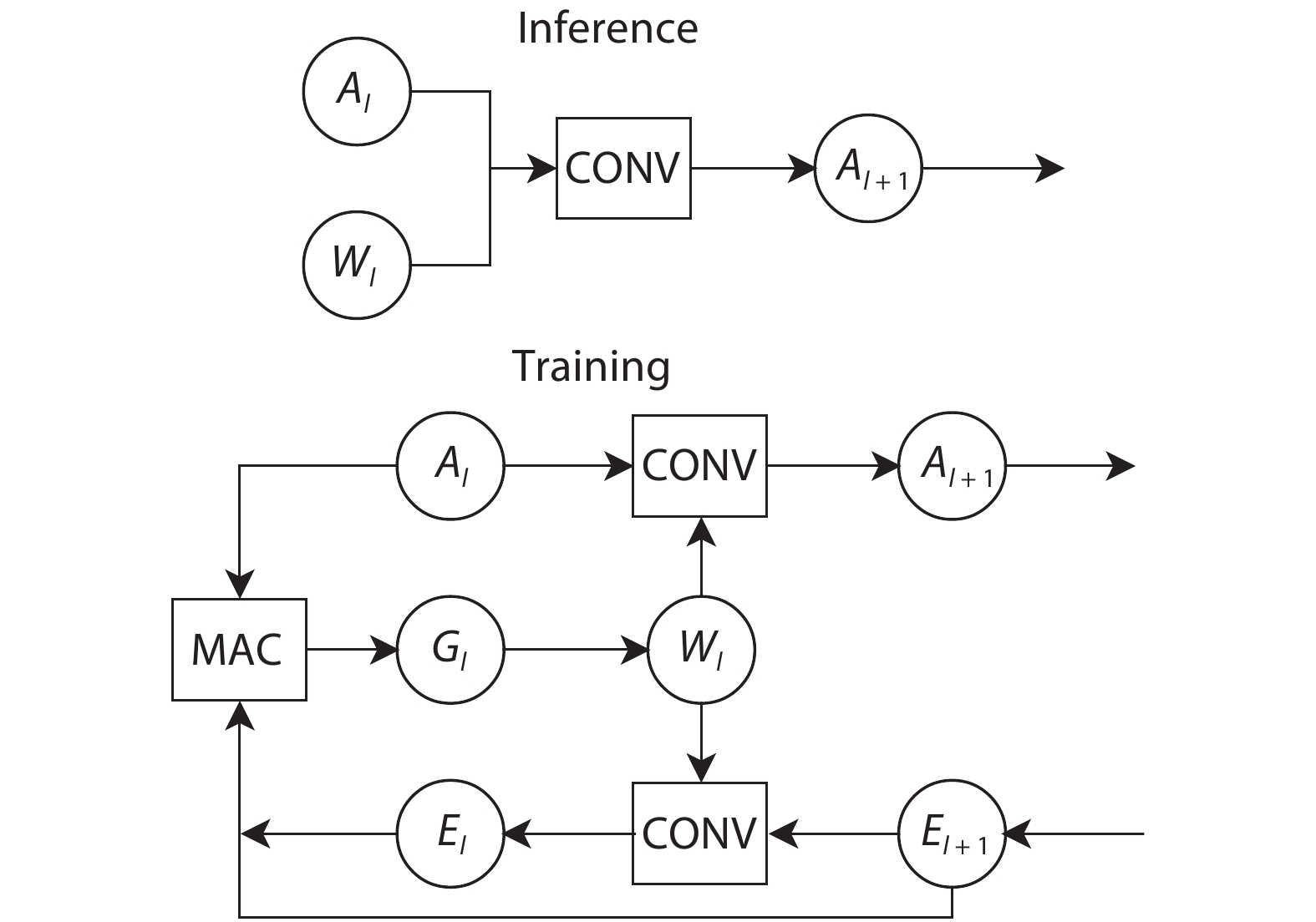
The training consists of forward propagation to compute the loss of the cost functions, and backward propagation to compute the gradients of the cost function, subsequently using gradients to update the model weights for learning desirable behavior. Unlike inference with only forward propagation, training with backward propagation is more computationally expensive and introduce additional operations for backward propagation.

Fig. 1 illustrates the overview of the inference and training of a convolutional layer. For a specific layer , the inference process with forward propagation simply convolves the input activations ( ) with the weights ( ) to generate the output activations for the next layer ( ). On contrast, the training process separately performs forward propagation to compute the errors using the loss function, and backward propagation to convolve the errors ( ) from the last layer with the current weights ( ) to calculate the errors to be propagated to the previous layer ( ). The backward propagation of training also compute the gradients ( ) with respect to the loss function using multiply–accumulate operation (MAC). These gradients update the current weights according to the chosen optimization algorithm like Adam^[21].

For better understanding, the pseudocode for training a convolutional layer is presented on Algorithm 1, which provides a precise description for the training process. The meaning of the notations can be found in Table 1, where the same set of notation is also followed in the rest of this paper.

Most FPGA accelerators mainly focus on the DNN inference acceleration^[22-27]. They^{[24, 28]} usually exploits image-level and layer-level parallelism extensively for efficient inference speedup. For training accelerators^[29-35], Geng et al.^[31] explore layer-level parallelism for training a model on multiple FPGAs in a pipelined manner. Li et al.^[32] study different reconfigurable communication patterns on a multi-FPGA cluster. Dicecco et al.^[33] study low-precision training with a reduced precision floating-point library. However, those accelerators usually deploy the inference architecture naively for training without considering the batch-level parallelism and additional backward operations, which may lead to undesirable performance.

Recently, some researchers^{[29, 36]} attempt to tackle the problem by distributing the DNN computations across a heterogeneous FPGA-CPU system. Moss et al.^[36] propose to perform the core GEMM operations on FPGAs and leave CPU for the remaining jobs. This solution works well on FPGA-CPU heterogeneous system but requires effective load balancing support for heterogeneous devices, since unpredictable communication cost between CPUs and FPGAs can make the FPGA-CPU cross communication a new bottleneck of the design. Based on our profiling in Section 8, the operations executed on CPU may require more computational time than FPGA acceleration of matrix multiplication.

With the objective of speeding up training, this paper studies the acceleration of entire training on a single FPGA, explores the parallelism in training batches, and provides an architecture suitable for bidirectional propagation. We propose a low-precision DNN training framework accelerated on a single FPGA platform. Compared to other frameworks, our proposed customizable FPGA design achieves about 10 times speedup over a CPU-based implementation and is about 2.5 times more energy efficient than a GPU-based implementation.

Our low-precision training algorithm is developed based on WAGE^[15], which is modified version for better FPGA implementation using shift-based linear mapping and hardware-friendly quantization. Our optimizations are illustrated here.

The basic idea of WAGE^[15] is to constrain four operands to low-bitwidth integers: weight and activation in forward propagation, error and gradient in backward propagation, using corresponding quantization operations , , , in computation flow to reduce precision. Experiments show stable accuracy can be obtained on multiple datasets. However, for hardware implementation, complex mathematical functions including logarithm, exponential operation which can be easily realized on CPU/GPU are hardly mapped on FPGA-implementation. Therefore, hardware-friendly customized operations are necessary for the accurate and efficient FPGA-based deep neural network training.

In order to quantize floating-point numbers to fixed-point number, k-bit linear mapping is adopted on WAGE^[15], where continuous and unbounded values are discretized with uniform distance :

$\begin{array}{l} \sigma(k) = 2^{(1-k)}, \quad k \in N_+ , \\ Q(x,k) = {\rm{Clip}}\{ \sigma(k) \times {\rm{round}} \left[\dfrac{x}{\sigma(k)}\right], -1 + \sigma(k), 1 - \sigma(k) \} .\end{array}$ ()

Here round function maps quantized floating-point number to nearest fixed-point number. Clip is the saturation function to clip unbounded values to .

Considering large hardware implementation overhead for floating-point operations, mathematical equivalent integer operations are introduced in our implementation, where the linear mapping is transformed into shifting from large data format (32-bit integers) to small integers ( -bit integers) which can be expressed as:

$ \begin{array}{l}\sigma(k) = 2^{(k-1)}, \quad k \in N_+, \\ Q(x,k,{\rm{shift}}) = {\rm{Clip}}\left\{ (x + {\rm{round\_value}} ) \gg {\rm{shift}},\right.\\ \qquad\qquad\qquad \left. -1 + \sigma(k), 1 - \sigma(k) \right\} , \\ {\rm{round\_value}} = 1 \ll ({\rm{shift}} - 1). \end{array} $ ()

Here we replace division operations used in float-point equations d with shift operations with an additional monolithic scaling factor shift for shifting values distribution to an appropriate order of magnitude. The scaling factor shift is obtained in WAGE^[15] by following equation.

$ \begin{array}{l} {\rm{shift}}(x) = {{\rm{round}}({\rm{log}}_2 x )} . \end{array} $ ()

With complex logarithm and exponential operation, the shift(x) requires extensive resources to be implemented on FPGA. To handle this problem, we fine-tune this formula, which is used to obtain the nearest power-of-two value from input , to obtain ceiling power-of-two value as follow:

$ \begin{array}{l} {\rm{shift}}(x) = {{\rm{ceil}}({\rm{log}}_2 x )}. \end{array} $ ()

After fine-tuning, the shift factor is obtained from smallest power-of-two value greater than , and can be re-expressed by bit-wise operations as follow:

$ \begin{array}{l} {\rm{shift}}(x) = ({\rm{leading1}}(x) + 1) . \end{array} $ ()

Here leading1 function detects the position of the most significant "important" bit and return the index of the most significant "important" bit only. After detailed experiments, the fine-tuning has no effect on the convergence of network training but more hardware-friendly for FPGA implementation.

The quantization operations consist of four operations , , , . Theses operations is responsible to quantize four training operands including weight , activation , error and gradient to low-bitwidth format.

Weights are initialized on software platform based on the initialization method of He et al.^[37], which can be formulated as:

$ \begin{array}{l} W \; U(-L, +L), \; L = {\rm{max}}\{\sqrt{6/n_{\rm {in}}}, L_{{\rm{min}}}\}, \; L_{{\rm{min}}} = 1 , \end{array} $ ()

where is the layer fan-in number, and the original limit is calculated to keep same variance between inputs and outputs of the same layer theoretically. The additional limit is a minimum value that the uniform distribution should reach.

For activation, the bitwith of activation would increase after computation. A filter-wise scaling factor is introduced for shifting values distribution to an appropriate order of magnitude, which can be obtained by following function:

$ \begin{array}{l} a_{\rm {shift}} = {\rm{log}}_2({\rm{max}}\{{\rm{shift}}(L_{\rm{min}}/L), 0\}). \end{array} $ ()

This factor is pre-defined constant for each layer determined by the network structure. Using this factor we can obtain the quantized activation using the following equation:

$ \begin{array}{l} a_{\rm{q}} = Q(a,k_{\rm{A}},a_{\rm {shift}}). \end{array} $ ()

Experiments from WAGE^[15] demonstrate the orientation of errors plays an important role on the converge performance during training. Therefore, orientation-based quantization scales errors into [–1,1] by dividing a shift factor as:

$ \begin{array}{l} e_{\rm{q}} = Q(e,k_{\rm{E}},{\rm{shift}}({\rm{max}}|e|)), \end{array} $ ()

where extracts the layer-wise maximum absolute value among errors. Since the shift value extracts the smallest power-of-two value for , an obvious optimization method is using "or" operations instead of max to improve the hardware performance.

$ \begin{array}{l} e_{\rm{q}} = Q(e,k_{\rm{E}},{\rm{shift}}({\rm{or}}|e|)) , \end{array} $ ()

where executes the bit-wise or operation on the layer-wise maximum absolute value among error.

Since we only preserve the relative value of the error after shifting, the gradients are shifted consequently. Here we first rescale the gradient with another scaling factor:

$ \begin{array}{l} g_{\rm{q}} = {\rm{Bernoulli}}\{ (\eta\times g ) \gg g_{{\rm{shift}}} \}, \\ g_{{\rm{shift}}} = {\rm{shift}}({\rm{or}}|g|)), \end{array} $ ()

where is learning rate which is constrained as power-of-two. So can also be represented by the corresponding shift value. Here gradients are quantized as errors by the bit-wise operation instead of the maximum function .

Bernoulli^[38] function was originally design in floating-point number system to stochastically sample fractional parts to either 0 or 1. The nature of the Bernoulli distribution is the larger number has higher probability to 1 and the smaller number has higher probability to 0. On contrast in integer system, Bernoulli function is stochastically rounding the shifting parts of quantized value, which is realized by a random number generator MersenneTwister, a widely-used general-purpose pseudorandom number generator^[39] to generate Limited range of random numbers according to shift data with uniform distribution. The MersenneTwister adds Bernoulli property by addition as following equation:

$ \begin{array}{l} g_{\rm{q}} = {\rm{Clip}}\left\{ (\eta\times g + {\rm{round\_value}}) \gg g_{{\rm{shift}}},\right.\\ \qquad \left. -\,1 + \sigma(k), 1 - \sigma(k) \right\}, \\ g_{{\rm{shift}}} = {\rm{shift}}({\rm{or}}|g|)) ,\\ {\rm{round\_value}} = {\rm{random\_int}}\;{\rm{mod}} (1\ll g_{{\rm{shift}}}), \end{array} $ ()

where is random numbers of 32-bit integer format.

For DNN training, the weights, activations, errors and gradients are too large to be stored completely in the on-chip memory, where only a portion of data can be cached on-chip while the remaining is kept off-chip. As the bandwidth between the on-chip and off-chip memory is limited, exploring an optimal data access pattern to for efficient bandwidth utilization is necessary for training.

Currently, the most widely-used data pattern for training on GPUs is referred as batch-channel-height-width (BCHW), which depicts the order of data dimensions in the memory space^[40], where the elements along the lowest dimension W are stored consecutively. An example of data represented in the BCHW pattern is shown on Fig. 2(a), whose corresponding data layout is illustrates in the DRAM in Fig. 2(c). But this pattern is difficult to fetch the elements from different batches in burst mode, because they are usually not stored consecutively in memory. Therefore, BCHW data pattern may under-utilize the bandwidth when exploring batch-level parallelism.

To handle the problem, we develop the channel-height-width-batch (CHWB) pattern to explore batch-level parallelism without compromising bandwidth utilization on FPGAs. As shown in Fig. 2(b), the elements from adjacent batches are allocated consecutively, which allows the memory interface to simultaneously read multiple training examples. In this manner, CHWB data pattern enables our accelerator to acquire all necessary input data with a single DRAM burst access, and greatly improve bandwidth utilization for FPGA accelerator.

Tiling is a common optimization technique to improve bandwidth utilization for DNN acceleration on resource-limited FPGA devices^[41]. The strategy partitions large input frames into smaller tiles of data, where each tile can be fitted into the on-chip memory of an FPGA. For training with some resource-intensive tasks such as matrix transpose, tiling strategy is necessary for their FPGA implementation.

For the CHWB pattern, we consider tiling along four data dimensions: batch tile , channel tile , filter tile and image tile , which correspond to the size of a tile along the dimension. Consider the input matrix transpose between the image dimension and channel dimension, as well as the weight matrix transpose between the channel dimension and filter dimension during training^[42], the image tile , the channel tile and the filter tile are all set to same value. In this case, two levels of parallelism are explored in our design: the batch-level parallelism and the image-level parallelism , which are controlled by the tiling parameters and respectively.

Taking convolution to explain how tiling technique works. In Fig. 3, the input matrix is stored using CHWB pattern 3-dimensions tiled blocks, while the weight matrix is stored with two-dimensional tiled blocks. In the forward propagation, the tiled input matrix and the tiled weight matrix are sequentially multiplied to obtain one output submatrix.

The tiling parameters and must be chosen carefully, since a larger tile size can improve performance by reducing the iterations of data transfers, but more on-chip memory resources are required for storing larger tiles. In Section 6. we will explore the optimization of the tile parameters on resource-limited FPGA.

In this section, we follow the idea of CHWB pattern and tiling technique to develop the architecture of our training accelerator.

A system overview of our FPGA-based training accelerator is presented on Fig. 4, which consists of a computation kernel, a global controller and a DDR controller for off-chip memory transfer. The computational kernel consists of a batch splitter, a set of processing elements (PEs) and a batch merger. When a stream of training batches arrives at the kernel, the splitter divides the stream into multiple parallel streams via shift registers to facilitate batch-level parallelism. The streams are then processed by the PEs in parallel. Each PE involves a general matrix multiplication kernel (GEMM kernel) or an auxiliary kernel to perform training operations. After processing, the streams are merged into a single output stream, then sent to the DDR controller. The global controller is responsible for controlling the behaviour of each computation kernel, including assigning memory addresses for loading/writing data through the DDR controller, enabling special operations required by particular layers, and controlling the direction of the data flow. The CPU sets the network configuration in the global controller before starting training.

Fig. 5 presents the architecture of the GEMM kernel, which provides a unified datapath to support the convolutional and fully-connected computations of the forward and backward propagation, as well as the gradient generation. This unified approach employ matrix multiplication to implement for these computations, where only the input/output matrix to/from the kernel needs to be changed. Therefore, we can avoid time-consuming dynamic reconfiguration^[29] or using separate kernels for different operations^[31].

Before any computation, the input data streams are stored in the input buffers, which are organized as a double buffer in order to overlap the data transfer and matrix transposition with the computation. As shown in Fig. 6, when the tile flows from the batch splitter to the input buffer, the tile is sent to the GEMM kernel for the computation. Note that the weight stream bypasses the batch splitter and enters the input buffers directly, as the weight data are shared by different tiles across the same batch.

The GEMM kernel fetches data from the input buffers to perform tiled matrix multiplication. The intermediate values during each iteration are stored in the output buffers for the next iteration. The final results are post-processed by the batch merger then transferred back to the DRAM. The details of the tiled matrix multiplication are shown in Algorithm 2. Noted that the shift factor of forward propagation is pre-defined while the the shift factor of backward propagation is obtained from output results. Therefore, the quantization function can be attached after forward propagation to reduce output bandwidth. On contrast, the output results maintain Int32/Int16 format during backward propagation as well as gradients generations, which require quantization with the help of auxiliary kernels.

In order to support different modes of operations for the forward propagation, the backward propagation and the gradient generation, the global controller dynamically re-configures the buffers and data flow on the datapath. Under the control of global controller, the input buffer can be configured to perform on-the-fly matrix transposition for the computation of backward propagation. Furthermore, the multiplexer can be switched to feed the different input streams to their corresponding processing elements, and the demultiplexer can be switched to direct the output stream to the appropriate postprocessing unit.

The auxiliary kernels accelerate supplementary operations with batch-level parallelism including im2col, col2im, max-pooling, reshape, summation, nonlinear functions and quantization as well as their backward counterparts (if necessary). These supplementary operations processed independently since they have no learnable weights and occupy only a small amount of total computation.

For various supplementary operations, various types of separate processing units is implemented to support them. In particular, the maxpooling units are responsible for computing the maximum value and corresponding index over a number of neighbor pixels, whereas the backward maxpooling units propagate errors the to chosen index of subgraphs. The im2col expands the input feature map into column vectors, and col2im accumulate column the vectors back to input feature map. The quantization units are designed for casting intermediate variables of errors and gradients generated during backward propagation and gradients generation to low bit-width quantized data (8-bit integer in our design). The summation units simply add two flows together and the reshape units change the location of data in buffers.

This section presents the design space exploration for optimizing the proposed DNN training accelerator. The performance of FPGA implementations is affected by factors including batch tiling size , image tiling size and bitwidth for training. The bitwidth is pre-defined while the two tiling sizes are decided by our optimization model. To maximize performance, we develop bandwidth modelling, resource modelling and performance modelling to enable design space exploration.

There are three kinds of hardware resources in FPGAs: LUT, Block RAM and DSP, which form the resource constraints of our design space. We present equations to estimate the utilization for each of them.

First, the resource consumption of the global controller and the DRAM controller is independent of the design parameters, while they are defined as , , .

Second, the resource consumption of the computational kernels is affected significantly by different design parameters. For example, BRAMs are utilized in the input buffers of GEMM kernels and their usage is given by:

$ \begin{array}{l} {\rm{BRAM}} = \dfrac{4 \times T_{\rm{B}} \times T_{\rm{I}}^2 \times (2\times L_{\rm{I}}) + 4 \times T_{\rm{I}}^2 \times L_{\rm{W}}}{{\rm{BRAM}}_{\rm{SIZE}}}, \end{array} $ ()

where the constants 4 are contributed by the double buffers for both the normal matrix and the transposed matrix.

The multiply-and-add units utilize the DSPs as

$ \begin{array}{l} {\rm{DSP}} = T_{\rm B} \times T_{\rm I} \times D_{\rm{mul}} + T_{\rm B} \times A_{\rm l} \times D_{\rm{add}} + T_{\rm B} \times D_{\rm{add}}, \end{array} $ ()

where and are the DSP usage of the multiplier and adder. is the level of tree adder in the computational kernel, which equals to .

Finally, an approximate regression model is proposed to estimate the resource consumption of LUT as it is difficult to predict statically:

$ \begin{array}{l} {\rm{LUT}} = T_{\rm B} \times T_{\rm I} \times \beta + T_{\rm B} \times \delta , \end{array} $ ()

where are linear function parameters pre-trained based on a specific platform.

There are three streams flowing from the DRAM to the GEMM kernels. In each cycle of convolution, one weight is read from the weight stream while input values are read from input frame stream. The results are accumulated in processing elements before iterations of the convolution are completed. When it comes to the fully-connected layer, additional weights are needed which increase the bandwidth requirement. Therefore, the theoretical maximum bandwidth requirements for computing the convolutional and fully-connected layers with frequency are:

$ \begin{array}{l} {\rm{BW}}_{\rm{CONV}} = ( T_{\rm{B}} \times L_{\rm{I}} + \dfrac{ T_{\rm{B}} \times T_{\rm{I}}} { N } \times L_{\rm{O}} + L_{\rm W}) \times f, \\ {\rm{BW}}_{\rm{FC}}= ( T_{\rm{B}} \times L_{\rm{I}} + \dfrac{ T_{\rm B} \times T_{\rm{I}}} { N }\times L_{\rm{O}} + T_{\rm{I}} \times L_{\rm{W}}) \times f, \end{array} $ ()

where , , are the bitwidth of the input frame, the output frame and the weight stream.

For the auxiliary kernel, the bandwidth requirements are relatively large compared to the small amount of computations performed. In general, it may take one or two input values to generate one or two output values, which handles up to 4 values in each cycle. As these operations benefit from batch-level parallelism, the bandwidth requirements have also multiplied times:

$ \begin{array}{l} {\rm{BW}}_{\rm{auxiliary}} = (2\times T_{\rm B} \times L_{\rm I} + 2\times T_{\rm B} \times L_{\rm O}) \times f. \end{array} $ ()

In each clock cycle, a GEMM kernel can accomplish matrix multiplication operations. Therefore for our batch-parallel architect with kernels, the total computational time under frequency is:

$ \begin{array}{l} {{T}}_{\rm{CONV}}= \dfrac{B \times C \times K \times F \times H \times W}{T_{\rm I} \times T_{\rm B} \times f}, \\ {{T}}_{\rm{FC}}= \dfrac{B \times C \times F }{T_{\rm I} \times T_{\rm B} \times f}. \end{array} $ ()

However, the above formulae are only valid for the sequential case. In fact, in order to support parallel computing, tiled matrices are filled with zero values which may affect the actual computational time. Therefore, the computational time is estimated as:

$ \begin{array}{l} T_{\rm{CONV}} = \dfrac{\lceil B \rceil ^{T_{\rm B}} \times \lceil C \times K \rceil ^{T_{\rm I}} \times \lceil F \rceil ^{T_{\rm I}} \times \lceil H \times W \rceil ^{T_{\rm I}} }{T_{\rm B} \times T_{\rm I} \times f}, \\ T_{\rm{FC}} = \dfrac{\lceil B \rceil ^{T_{\rm B}} \times \lceil C \rceil ^{T_{\rm I}} \times \lceil F \rceil ^{T_{\rm I}} }{T_{\rm B}\times T_{\rm I}\times f} , \\ \lceil X \rceil ^{T} = {\rm{ceil}}(X / T) \times T, \end{array} $ ()

where function means mapping to the least multiple of greater than or equal to , which indicates that these formulae are identical only when tiling sizes are set as factors of the corresponding parameters.

On the other hand, in each cycle of the auxiliary kernel, frames batches can be handled simultaneously, where the computational time of auxiliary kernels is:

$ \begin{array}{l} T_{\rm{auxiliary}} = \dfrac{\lceil B \rceil ^{T_{\rm B}} \times C \times H \times W }{T_{\rm B} \times f,} \end{array} $ ()

Benefited from our dataflow architecture, the transmission time of the computational kernels can be overlapped by the communication time.

By evaluating the performance of every combination based on the above models, a single-objective optimization tool can be built for minimal execution time as:

$\begin{array}{l} {\rm{Minimize\;Time}} = T'_{\rm{CONV}} + T'_{\rm{FC}} + T'_{\rm{auxiliary}} ,\\ {\rm{where}}\left\{ \begin{array}{l} {\rm{LUT}} + {\rm{LUT}}_{\rm{fix}} \leqslant {\rm{LUT}}_{\rm{limit}} , \\ {\rm{BRAM}} + {\rm{BRAM}}_{\rm fix} \leqslant {\rm{BRAM}}_{\rm{limit}}, \\ {\rm{DSP}} + {\rm{DSP}}_{\rm{fix}} \leqslant {\rm{DSP}}_{\rm{limit}} , \\ {\rm{BW}} \leqslant {\rm{BW}}_{\rm{limit}}, \\ \end{array} \right. \end{array} $ ()

where , , , are limited on-chip resources, and + + are the expected computation time for a specific network description.

For our proposed dataflow architecture, we present DarkFPGA, a hardware/software co-designed FPGA framework for effective training. DarkFPGA framework is built with scalable accelerator architecture which is software-definable to support various DNN networks and different parallel levels through deploying different FPGA bitstreams, where a multi-level parallelism scalable FPGA design is developed. Moreover, a optimizing tool is included to produce optimised design for optimised performance based on user constraints.

We automate the process of exploring design parameters for the DarkFPGA framework, which accelerates the entire training process with a unified module on FPGA. Our tool can receive a network description and a training dataset to produce the most suitable parameters for the accelerator. The overview of our DarkFPGA framework and optimizing tool are illustrated in Fig. 7 with six stages:

(1) Parse network description. The tool predicts optimized parameter values and selects a suitable FPGA bitstream to configure hardware.

(2) Allocate device DRAM space for the activations, weights, errors and gradients.

(3) Initialize weights and transfer them to DRAM.

(4) Fetch and transfer the training samples to DRAM. Data reorganization is used to convert training samples into the CHWB sequence.

(5) Launch FPGA acceleration.

(6) Train neural network iteratively. Transfer loss and accuracy information back to the host for each complete training batch.

We evaluate our framework on the Maxeler MAX5 platform, which consists of a Xilinx ultrascale+ VU9P FPGA. Three 16 GB DDR4 DIMMs are installed on the platform with a maximum bandwidth of 63.9 GB/s. Our hardware accelerator works at 200 MHz. Maxcompiler 2019.1 and Vivado 2018.3 are used for synthesis and implementation. The VGG-like network^[43] trained on the Cifar10^[1] dataset is evaluated in the following training experiments. Differ form the conference version of this paper^[20], we use INT8 weights instead of ternary weight during training. Although the use of INT8 weights cause inevitable degradation in training performance, it is able to obtain more stable accuracy performance for training.

Noted while our implementation are able to achieve the massive parallelization with dataflow architecture, it may have difficulty in making the timing closure for a high clock frequency, or even passing the place and route. This is partly because these direct interconnects become long wires when the DSP blocks are distributed among the whole FPGA chip, and large-scale data reuse between DSP blocks introduces large fan-out^[44]. Moreover, the timing closure get worse on Xilinx ultrascale+ VU9P FPGA which enables multiple super-logic regions (SLR) design. In this case, signal paths between two SLR may introduce large delays and significantly impact timing. DarkFPGA tackles the timing issue for two major optimization. First, a multiple level of pipelining registers is inserted after high fan-out data stream as a balanced tree to limits the fan-out it can have. Second, the GEMM Kernel of DarkFPGA is forced to be divided into two parallel submodules, which are assigned to a super-logic regions (SLR). These signal interconnects of GEMM Kernel are limited within their corresponding super-logic regions (SLR).

Based on the discussions in Section 5 and Section 6, the performance of DarkFPGA is significantly determined by the tile sizes ( ). Therefore, the selection of tile parameters is analyzed here under the network configuration shown in Table 2.

The batch tile is crucial for maximising performance, which is bounded by the training batch size. Consider that the commonly used batch size is 128, the selection of batch tile for exploration is constrained among (32, 64, 128). Also, the image tile is mainly related to the computational times and , which depends on the network parameters , , and . According to Table 2, the selection of image tile is constrained among (16, 32, 64). Due to the requirements of matrix transposition operations, the batch tile should be greater than or equal to image tile . Therefore the design space ( , ) under evaluation is constrained within (128, 64), (128, 32), (128, 16), (64, 64), (64, 32), (64, 16), (32, 32), (32, 16), (16, 16). In particular, the design space (128, 64) is removed from evaluation for hardware resource limitation.

The corresponding performance and resource consumption under different design parameters ( , ) is illustrated in Fig. 8. As shown in Figs. 8(a) and 8(b), the design space ( , ) changes from (128, 32) to (32, 16) as the performance decreases. We can find that the most critical factors that affect the performance are the multiplication of two tiling size ( ). The reason is that, according to our performance model, the computational time for matrix multiplication operations are accelerated by ( ) times, which domain the training process. And the secondary influencing factor is batch-level parallelism ( ). This is because the auxiliary operations are only accelerated by times, with no relationship about . Finally, Fig. 8(c) shows the relation between DSP utilization and performance, indicating that our design space is bounded by DSP resources.

Therefore, we customize a DarkFPGA design to determine the optimal implementation of the training accelerator when , .

Some of the existing FPGA accelerators rely on heterogeneous computing to handle auxiliary operations^{[36, 45]}. To quantitatively compare the performance discrepancies between heterogeneous and homogeneous computing, our DarkFPGA framework is revised to implement heterogeneous computation across an FPGA-CPU heterogeneous system, which is achieved by delivering auxiliary operations to CPU and removing the auxiliary kernels.

In this experiment, the tiling size is set to ( ). Fig. 9 illustrate the experiment results which show that homogeneous computing can achieve significantly higher performance on our DarkFPGA framework. Based on the comparison between CPU homogeneous system and CPU+FPGA heterogeneous system (Fig. 9(a) versus Fig. 9(b)), heterogeneous computing can effectively improve the performance of GEMM, but other parts of the training would become a new computing bottleneck. This problem can be addressed with a homogeneous FPGA system, accelerating everything by batch-parallelism to achieve over 10 times speedup (Fig. 9(b) versus Fig. 9(c)). This experiment clearly showcases the benefits of implementing the entire training process on the FPGA.

Note that using multi-threaded or high-performance CPU can significantly improve heterogeneous computing performance. However their high power consumption brings a tough challenge for embedded DNN applications.

Here we compare the performance of DarkFPGA with other platforms like GPU and CPU. All software results are running on an Intel Xeon X5690 CPU (6 cores, 3.47 GHz) and an NVIDIA GeForce GTX 1080 Ti GPU. After finishing the same number of batches, all platforms achieve similar accuracies. Unfortunately, GeForce GTX 1080 Ti does not have native int8 support, we evaluate the GPU performance by limiting the range of float32 number system, instead of actual GPU low-precision training.

Table 3 shows the performance and power consumption, as well as other important metric on different platforms. DarkFPGA can achieve over 200 times speedup over a CPU-based implementation of Darknet and is 2 times slower than a GPU-based implementation of Darknet on overall performance. The average power consumption (13.5 W) of FPGA is obtained by the Maxeler performance monitoring tools. By multiplying time and power consumption, our FPGA-based design is 5 times more energy efficient than GPU implementation of Darknet.

Note that Darknet is a lightweight neural network framework for fast iterative design, which limits the overall performance of GPU and CPU. For fair comparison, we evaluate the training performance on TensorFlow^[46] using multi-threaded acceleration for CPU and cuDNN^[47] acceleration for GPU, as shown in brackets. It shows that DarkFPGA achieves 10 times speed up over CPU-based implementation and 2.5 times more energy efficient than GPU implementation on TensorFlow.

Finally, comparisons between out DarkFPGA and other FPGA training accelerators are conducted, in terms of resource utilization, performance and throughput and on Table 4. Since many important matrices are not provided and the models for training are different, comparison between different FPGA-based training accelerator in a fair is extremely difficult and not straightforward. Even in such situation, our DarkFPGA accelerator still show desirable performance. Our design outperforms FPDeep^[31] in term of performance per FPGA. Accelerator from DiCecco et al.^[33] outperform our accelerator in throughput by training small network similar to LeNet-5^[1]. Moreover, in comparison to^[35], a lightweight FPGA training accelerator, our DarkFPGA maintains a high throughput when training more smaller network VGG-16^[43] compared with^[35]. A work from^[34] achieves much higher throughput than our implementation by pruning over 90% weights and 50% activation during training process, whose performance can be 4× faster than GPU.

These comparisons can somehow show that our DarkFPGA has the capacity to train deep neural network. Our analyses show that the improvement of performance comes from FPGA-based batch-level parallelism. In particular, the dataflow architecture allows us to fully exploit the advantages of batch-level parallelism and maximize throughput with the help of dataflow programming language^[19].

This work proposes DarkFPGA, a novel FPGA framework for efficient training of deep neural networks, with a customized low-precision DNN training algorithm. The DarkFPGA accelerator explores batch-level parallelism, which provides efficient training acceleration for both forward and backward propagation on a homogeneous FPGA system. Optimization strategies such as batch-focused data sequence CHWB and tiling strategies are employed to improve overall performance. Furthermore, an optimization tool is developed for determining the optimal design parameters for a specific network description. Future work includes applying DarkFPGA to multi-FPGA clusters, exploring mixed precision and binarised training, and supporting cutting-edge network functions like group normalization and depthwise convolution.