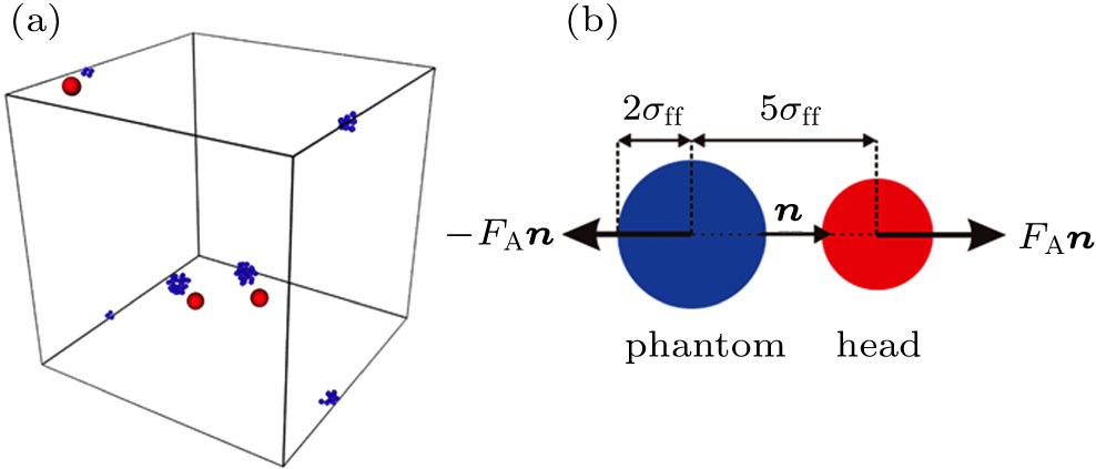
Fig. 1. (a) A snapshot of the simulation showing a dilute suspension of three active particles in the simulation box. The red particles are the head particles and the blue particles are the fluid particles in the phantom regions. Fluid particles out of the phantom regions are not shown here. Due to the periodic boundary conditions, the fluid body of one active particle is separated into four parts. (b) The ABP modeled in this work. A force dipole is exerted on the head particle and the phantom region of fluid to model a pusher.

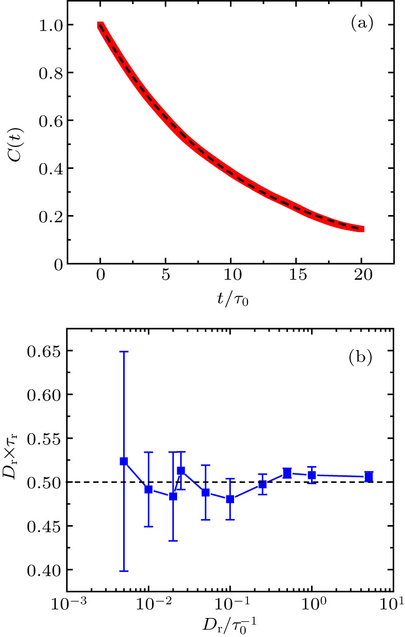
Fig. 2. (a) Exponential decay of the orientational time correlation function C(t) for Dr=0.05τ0−1. The red solid line represents the numerical result and the black dashed line represents the exponential fitting with τ_r = 10.32τ₀. (b) The product D_r × τ_r plotted for different values of D_r in units of τ0−1. Note that for small D_r, τ_r is large and leads to large statistical error in a limited time duration.

Fig. 3. (a) Gaussian distribution of the axial velocity w_A, plotted for different values of rotational diffusivity D_r (in units of τ0−1) and applied force F_A (in units of εffσff−1). (b) The active velocity v_A plotted as a function of the applied force F_A for Dr=0.01τ0−1 and 0.02τ0−1.

Fig. 4. Dependence of the standard deviation σ_A on the size of ABP.

Fig. 5. Trajectories of a PBP and three ABPs with l_A = 0.18σ_ff from τr=1τ0,vA=0.18σffτ0−1, l_A = 1.125σ_ff from τr=25τ0,vA=0.045σffτ0−1, and l_A = 4.5σ_ff from τ_r = 50τ₀, vA=0.09σffτ0−1. Each trajectory includes 100 frames with a time duration of 25τ₀.

Fig. 6. (a) MSD for PBPs (solid line), with D_T found to be 0.015σff2τ0−1 through a linear fitting (dashed line). (b) MSD for three ABPs with different values of D_r (in units of τ0−1) and F_A (in units of εffσff−1). In each case, the solid line represents the simulation data and the dashed line of the same color represents the corresponding linear fitting.

Fig. 7. MD simulation results for the dependence of D_A on vA2 for Dr=0.01τ0−1 and 0.02τ0−1. From the linear fitting (dashed lines), the prefactor α in DA≃αvA2τr is found to be 0.274 for Dr=0.01τ0−1 and 0.252 for Dr=0.02τ0−1.

Fig. 8. The equilibrium PDF g(r) of the confined PBP for k=εffσff−2.

Fig. 9. Evolution of the PDF g(r) with the increase of R₁. (a) The Boltzmann-type distribution for R₁ = 0.125. (b) A distribution slightly deviating from the Boltzmann-type for R₁ = 0.25. (c) A distribution exhibiting a plateau in the central region for R₁ = 0.5. (d) A bimodal distribution for R₁ = 1 with the accumulation of probability near r = ± r_B. Here the red line represents a fitting of the Boltzmann-type and the gray region is bounded by r = ± r_B.

Fig. 10. The PDF g(r) and marginal PDF f(x). (a) g(r) for R₁ = 0.5. (b) f(x) for R₁ = 0.5. (c) g(r) for R₁ = 2.5. (d) f(x) for R₁ = 2.5. In (b) and (d), f(x) directly measured in simulations (represented by solid circles) is compared to that obtained from g(r) by the use of Eq. (23) (represented by solid line), with good agreement.

Table 1. Comparison between D_AC and D_AF.