Author Affiliations
College of Physics and Electronic Engineering, Northwest Normal University, Lanzhou, Gansu 730070, Chinashow less
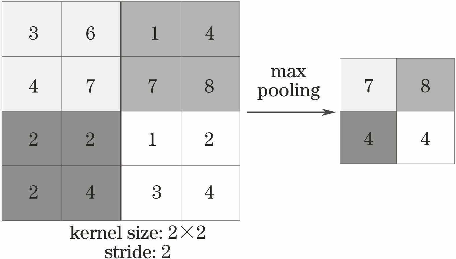
Fig. 1. Maximum pooling schematic
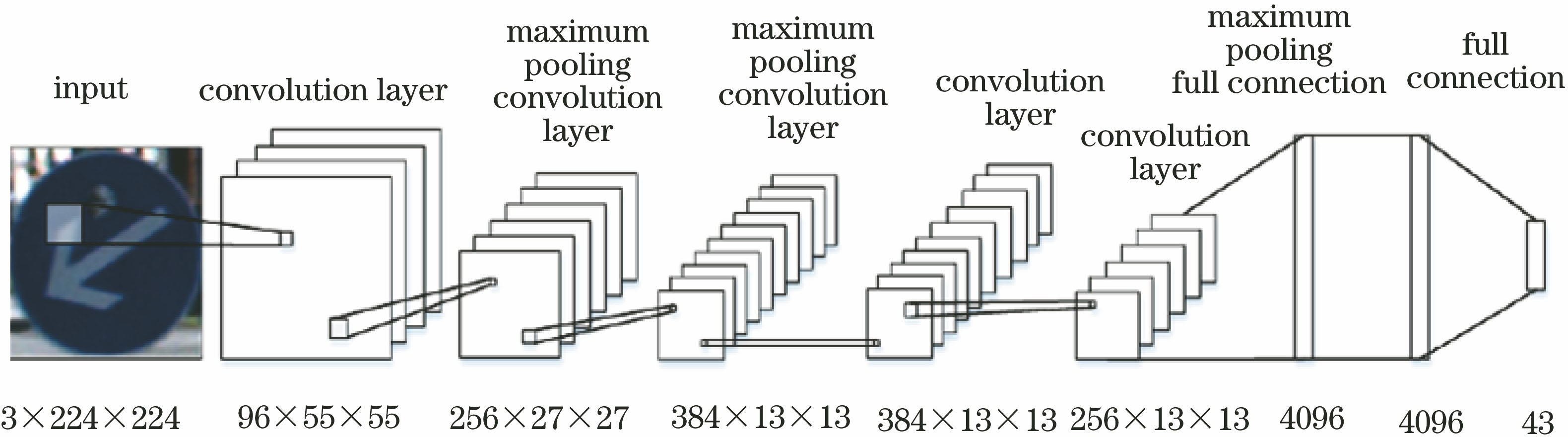
Fig. 2. Basic structure of AlexNet network
Fig. 3. Neural network contrast diagrams. Three-level neural network with (a) unused and (b) used dropout
Fig. 4. Structure diagram of improved AlexNet model
Fig. 5. Experimental flow chart
Fig. 6. Visualization of the coiling layer operation
Fig. 7. Contrast diagrams of (a) Accuracy and (b) loss
| Layer | Layerinput | Convolution kernel | Convolutionoutput | Pooling | Pooledoutput | Layeroutput |
|---|
| Size | | | Number | Step | Pad | Size | Mode |
|---|
| L1(conv1+pool1) | 48×48×3 | 3×3 | 84 | 1 | 1 | 48×48×84 | 2×2 | Max | 24×24×84 | 24×24×84 | | L2(conv2+pool2) | 24×24×84 | 3×3 | 125 | 1 | 1 | 24×24×125 | 2×2 | Max | 12×12×125 | 12×12×125 | | L3(conv3) | 12×12×125 | 3×3 | 250 | 1 | 0 | 10×10×250 | — | — | — | 10×10×250 | | L4(conv4) | 10×10×250 | 3×3 | 500 | 1 | 1 | 10×10×500 | — | — | — | 10×10×500 | | L5(conv5+pool5) | 10×10×500 | 3×3 | 250 | 1 | 0 | 8×8×250 | 2×2 | Max | 4×4×250 | 4×4×250 | | L6(conv6) | 4×4×250 | 3×3 | 250 | 1 | 0 | 2×2×250 | — | — | — | 2×2×250 | | L7(conv7) | 2×2×250 | 2×2 | 500 | 1 | 0 | 1×1×500 | — | — | — | 1×1×500 | | L8(Full) | 1×1×500 | — | — | — | — | — | — | — | — | 1000 | | L9(Full) | 1000 | — | — | — | — | — | — | — | — | 1000 | | L10(Softmax) | 1000 | — | — | — | — | — | — | — | — | 44 |
|
Table 1. Model setting of improved AlexNet network
| Model | AlexNet model | Improved model without dropout | Improved model with dropout |
|---|
| Test sample error number | 196 | 173 | 58 | | Test error rate | 0.040 | 0.035 | 0.012 |
|
Table 2. Impact of dropout on the model
| Algorithm | Trainingtime /h | Parameter consumptionmemory /MB | Identifying eachimage time /ms | Recognitionaccuracy /% |
|---|
| AlexNet model | 173 | 228.2 | 158 | 95.568 | | Improved model | 16 | 21 | 40 | 96.875 |
|
Table 3. Algorithm classification ability analysis
| Algorithm | Training time /h | Parameter consumption memory /MB | Recognition accuracy /% |
|---|
| Improved model | 16 | 21 | 96.875 | | Contrast model 2 | 21 | 21.7 | — | | Contrast model 1 | — | 21.2 | 93.750 |
|
Table 4. Algorithm comparison and analysis
| Algorithm | Classification time /ms | Accuracy rate /% |
|---|
| HOG+SVM algorithm of Ref. [17] | 176 | 95.68 | | ANN | — | 89.63 | | Random forests | — | 96.14 | | Improved model algorithm | 40 | 96.875 | | Algorithm of Ref. [1] | 275 | 99.01 | | Algorithm of Ref. [6] | 152 | 98.57 |
|
Table 5. Comparison of different methods in GTSRB dataset recognition results
| Type | Test sample number | Correct recognition number ofAlexNet model | Recognition accuracyrate of AlexNet model /% |
|---|
| Motion blur | 30 | 22 | 73.3 | | Background interference | 51 | 43 | 84.3 | | Light (weather) | 30 | 25 | 83.3 | | Shooting angle | 30 | 26 | 86.6 |
|
Table 6. Identification of AlexNet model under real environmental conditions
| Type | Test sample number | Correct recognition number ofimproved model | Recognition accuracy rate ofimproved model /% |
|---|
| Motion blur | 30 | 23 | 76.6 | | Background interference | 51 | 45 | 88.2 | | Light (weather) | 30 | 27 | 90.0 | | Shooting angle | 30 | 28 | 93.3 |
|
Table 7. Identification of improved model under real environmental conditions