
Fusheng Sun, Xie Han. Super-Resolution Algorithm Based on Precise Color Vector Constraint of Light Field Camera[J]. Acta Optica Sinica, 2019, 39(3): 0304001
- Acta Optica Sinica
- Vol. 39, Issue 3, 0304001 (2019)
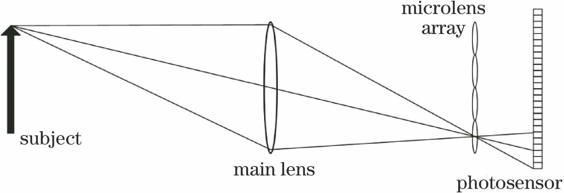
Fig. 1. Principle diagram of optical field imaging
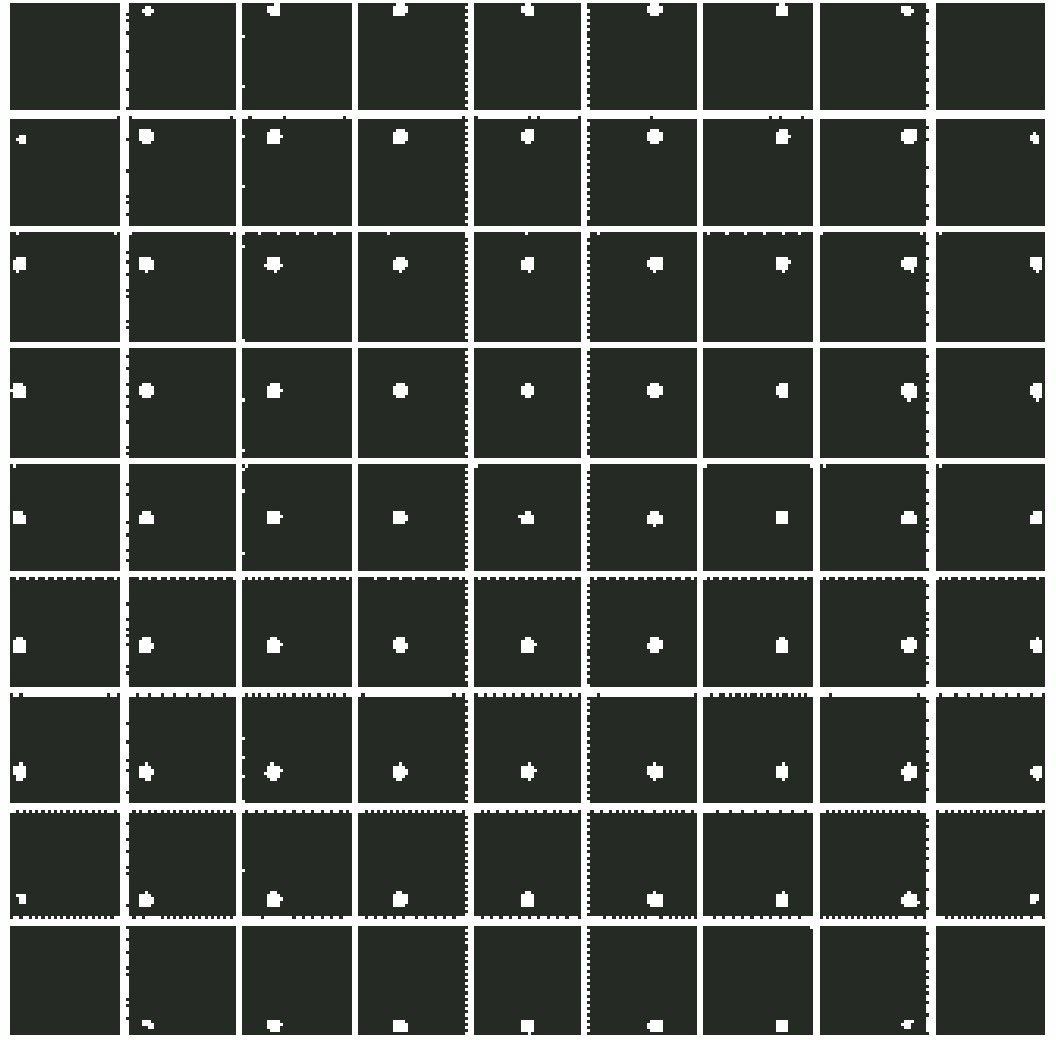
Fig. 2. Measured results of PSF of LYTRO camera
Fig. 3. Hexagonal RST coordinate system
Fig. 4. Distribution and location diagram of diffusion function points (a) and local magnification diagram (b)
Fig. 5. Distribution of color filters and diffusion function points
Fig. 6. Pyramid model
Fig. 7. Pyramid algorithm model of LYTRO camera
Fig. 8. Algorithm flow chart
Fig. 9. Original image information collected by LYTRO camera. (a) Image 1; (b) image 2
Fig. 10. Experimental results and local enlargement of 4 algorithms
Fig. 11. Color recovery results of two sets of images. (a) Bilinear algorithm; (b) Lu's algorithm; (c) adaptive algorithm; (d) proposed algorithm
Fig. 12. Original image and sub-aperture images. (a) Original image; (b) sub-aperture image; (c) 7×7 sub-aperture images
Fig. 13. Original image and local magnified images. (a) Original image; (b) local magnification image 1; (c) local magnification image 2; (d) local two times enlarged image 3
Fig. 14. Experimental comparison of algorithms. (a) Toolbox W/O rectification+dual three-time on-sample; (b) toolbox W/O rectification+super-resolution; (c) document algorithm[25]; (d) proposed algorithm
|
Table 1. Diffusion function point coordinates of different layers
| ||||||||||||||||||||||||||||||||||||||||||||||||||||||||||||||||
Table 2. Color filter distribution mode
|
Table 3. Image 1 evaluation data
|
Table 4. Image 2 evaluation data

Set citation alerts for the article
Please enter your email address
© Copyright 2018-2021 | Chinese Laser Press. All Rights Reserved 沪ICP备15018463号-20