• Chinese Optics Letters
  • Vol. 19, Issue 8, 081101 (2021)
Zhenming Yu, Zhenyu Ju, Xinlei Zhang, Ziyi Meng, Feifei Yin, and Kun Xu*
Author Affiliations
  • State Key Laboratory of Information Photonics and Optical Communications, Beijing University of Posts and Telecommunications, Beijing 100876, China
  • show less
    DOI: 10.3788/COL202119.081101 Cite this Article Set citation alerts
    Zhenming Yu, Zhenyu Ju, Xinlei Zhang, Ziyi Meng, Feifei Yin, Kun Xu. High-speed multimode fiber imaging system based on conditional generative adversarial network[J]. Chinese Optics Letters, 2021, 19(8): 081101 Copy Citation Text show less

    Abstract

    The multimode fiber (MMF) has great potential to transmit high-resolution images with less invasive methods in endoscopy due to its large number of spatial modes and small core diameter. However, spatial modes crosstalk will inevitably occur in MMFs, which makes the received images become speckles. A conditional generative adversarial network (GAN) composed of a generator and a discriminator was utilized to reconstruct the received speckles. We conduct an MMF imaging experimental system of transmitting over 1 m MMF with a 50 μm core. Compared with the conventional method of U-net, this conditional GAN could reconstruct images with fewer training datasets to achieve the same performance and shows higher feature extraction capability.

    1. Introduction

    Endoscopes are the devices that acquire images or other information through thin tubular structures, which have gradually developed into popular tools in medical and industrial fields[1]. Optical fiber bundles consisting of many single mode fiber cores are widely applied in endoscopes for image transmission[2]. However, the imaging resolution of the fiber bundle suffers from the coupling of light between adjacent cores when the cores are not sufficiently spaced from the others. With the increasing demand for imaging in medical and other fields, the imaging system with both higher resolution and smaller access diameter is very urgent. Multimode fibers (MMFs) own a large number of transmittable modes for unparalleled information transport and ultra-thin shape, which makes single fiber imaging possible. However, due to the strong mode coupling and interference within the MMFs, the images cannot be obtained directly. When the modulated coherent light passes through the MMF, a variety of transmission modes are excited and coupled with each other, which leads the received images at the distal end to become random speckle patterns. Moreover, the local defects along the MMFs also cause mode coupling and inter-mode interference, and the speckle patterns can be formed even after transmitting over a few millimeters[3,4]. Therefore, the main challenge of MMF imaging is how to reconstruct the original images from speckle patterns.

    Some approaches developed from computational imaging[5,6] such as phase conjugation, digital scanning, and holographic technique have been used to address the issues in MMF imaging systems[710]. However, these approaches are almost based on calibration, which are difficult in practical applications due to the low speed. Deep learning showed the potential to speed up the image reconstruction of MMFs and improve the robustness of environment. By training a deep neural network (DNN) with a large amount of captured data, the images transmitted through MMFs can be recovered very fast [∼milliseconds (ms)] by the DNN, and this process is calibration free[11,12]. U-net, which is powerful for image segmentation and restoration, has been verified to provide decent results for the image reconstruction from the MMF speckles. However, the conventional training strategy, i.e., using L2 loss functions, usually requires tens of thousands of image pairs for training, which brings a challenge for the training data acquisition.

    Generative adversarial networks (GANs) are utilized to optimize the DNN method. GAN was first proposed to get the natural image distribution from a random vector[13]. However, the GAN model uses an extensive training method during training, where all training samples are fed into the model for training without constraints. Therefore, the GAN model is uncontrollable when it is used for image generation, which leads to the generated image's unpredictability. A framework of conditional GAN was proposed by conditioning on an input image and generating a corresponding output image, which shows high performance in image-to-image translation tasks[14]. In this paper, we explore a new training strategy, which employs the framework of conditional GAN to recover the images transmitted through MMFs.

    2. Operating Principle

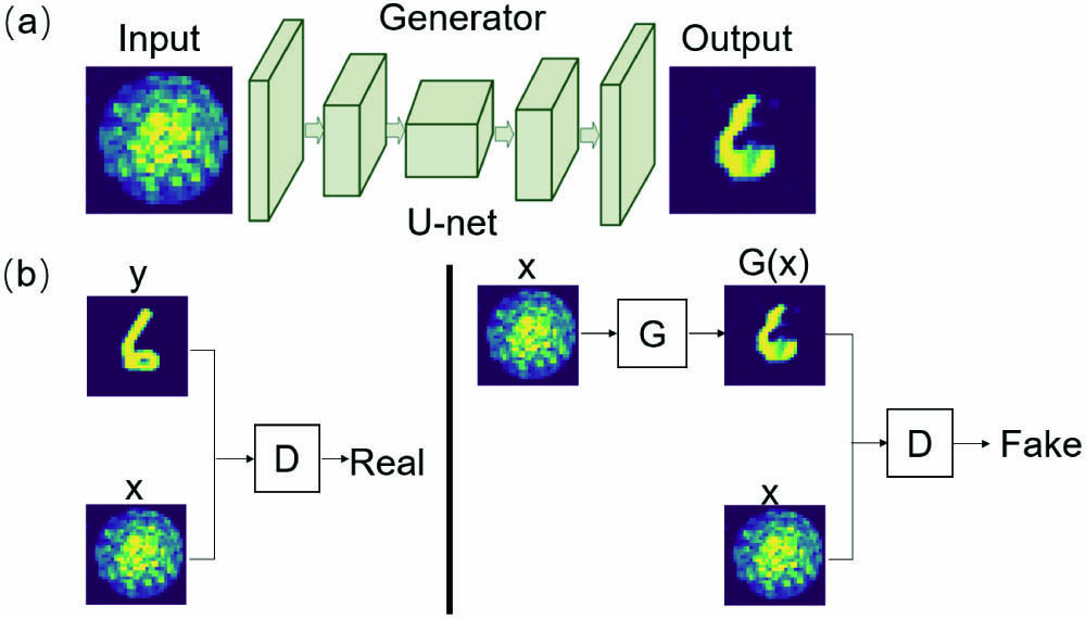
    The structure of the conditional GAN is shown in Fig. 1. Figure 1(a) is the network of the generator, which is a U-net in essence. The sizes of the input layer and output layer are determined by the resolution of the input image. The generator is divided into a contraction path and an expansion path in the network structure setting. The discriminator is a convolutional neural network. The input of the discriminator is the ground truth or the output image of the generator splicing with a corresponding speckle pattern, which follows the idea of conditional GANs, as shown in Fig. 1(b). The generator is trained to confuse the discriminator, which aims to make the discriminator fail to distinguish the output of the generator from the real images, while the discriminator is trained to distinguish the output of the generator as fake as far as possible. Unlike the discriminator in the conventional GAN, which determines whether the image generated by the generator matches the distribution of the real sample set, the function of the discriminator in this conditional GAN is to determine whether the image generated by the generator is the same as the label image of the real sample set. The objective of the conditional GAN is defined as[14]LcGAN(G,D)=Ex,y[logD(x,y)]+Ex,z{log{1D[x,G(x,z)]}},where x is the received speckle pattern, y is the ground truth, and z is the random noise introduced in the dropout layer of the generator. The generator G aims to minimize the objective, while the discriminator D aims to maximize it. In addition, a traditional loss L1 is also applied to make the generator produce the images close to the target images and reduce image blur, which is defined asL1=Ex,y,z[yG(x,z)1].

    Structure of the conditional GAN; (a) architecture of the generator; (b) principle of the discriminator. G, generator; D, discriminator.

    Figure 1.Structure of the conditional GAN; (a) architecture of the generator; (b) principle of the discriminator. G, generator; D, discriminator.

    Therefore, the final objective is[14]G*=argminGmaxDLcGAN(G,D)+λL1(G),where λ is a hyperparameter to balance the effects of the discriminator and L1 on generator training.

    3. Experimental Setup and Results

    The experiment setup is built as shown in Fig. 2 in order to get training data. A He–Ne laser (Thorlabs HNL210LB) operating at 632.8 nm generates a narrow laser beam. The laser beam illuminates a 1280×768 pixels digital micromirror device (DMD, V-7001, VIALUX) after transmitting through an optical expander (Edmund #2186) and an attenuator (NDC-100C-4M). The DMD modulates the gray-scale images onto the incident beam in amplitude by controlling the deflection of the internal micromirror. Then, the beam is coupled into a stable 1-m-long MMF (50-µm-core, Thorlabs) by the microscope objective lens (OBJ1, PLN 40× objective and single port tube lens, Olympus) and magnified by OBJ2 (the same as OBJ1). After that, the output speckle patterns are captured by a 1280×768 pixels CCD camera (PL-D721, PixeLINK).

    Experiment setup. DMD, digital micromirror device; OBJ, microscope objective lens; MMF, multimode fiber; CCD, charge-coupled device.

    Figure 2.Experiment setup. DMD, digital micromirror device; OBJ, microscope objective lens; MMF, multimode fiber; CCD, charge-coupled device.

    The Modified National Institute of Standards and Technology (MNIST) database and Fashion-MNIST database are used as input datasets, respectively. The images with a resolution of 28×28 pixels are padded to 32×32 pixels as the ground truth. The input images are then adapted to the 1024×768 pixels DMD by the operation of zero-padding and up-sampling. We can acquire one 512×512 pixels speckle pattern for every single image displayed on the DMD. Finally, the speckle patterns are resized into 32×32 pixels in the MNIST dataset and 128×128 pixels in the Fashion-MNIST dataset to facilitate subsequent processing.

    U-net has been proved to solve the image reconstruction problem with the MNIST dataset in MMF imaging system. In this conditional GAN, the structure of the generator is similar to the U-net, as shown in Fig. 3, which contains a down-sampling unit and an up-sampling unit. The down-sampling unit is made of several stride convolutional layers, which uses rectified linear units (ReLU) as the activation function. The features of the input image are concentrated in the bottleneck layer with a resolution of 1×1×256. The up-sampling unit is distributed symmetrically with the down-sampling unit, which has several deconvolutional layers. Skip connections are added between the down-sampling layers and the up-sampling layers with the same size. Due to the higher complexity of the Fashion-MNIST dataset, the resolution of the input speckle pattern and the depth of the network are increased. We use an asymmetric U-net-like network with input resolution of 128×128×1 and out resolution of 32×32×1 as the generator. At the same time, the resolution of the bottleneck layer is set to 2×2×512 to prevent overfitting caused by an excessively deep network.

    Structures of generator in the (a) MNIST experiment and (b) Fashion-MNIST experiment.

    Figure 3.Structures of generator in the (a) MNIST experiment and (b) Fashion-MNIST experiment.

    The discriminator is a convolutional neural network, which is shown in Fig. 4. The input is the speckle pattern concatenated with the image generated by the generator or the ground truth. The 32×32×2 input is followed by several convolutional layers. Finally, an eigenmatrix is output for discrimination. When the input contains the ground truth, the label is set to all ones, indicating that the input is real. If not, it is set to all zeros indicating that the input is fake.

    It is known that an image often has a low-frequency part and a high-frequency part. L1 in Eq. (2) could enforce correctness at the low frequencies[15]. In order to process the high-frequency part, a discriminator architecture called “PatchGAN” is applied, which divides the whole image into small patches and discriminates the authenticity of each patch, respectively[14]. The patch corresponds to the receptive field of the convolutional neural network[16]. The larger receptive field is implied to the larger area of the image map pixels, which better reflects the global and holistic areas. The smaller receptive field is implied to the smaller area of the image map pixels, which can reflect more locality and detail. Therefore, the larger value of the patch leads to the deeper discriminator network and higher discriminating ability in the low-frequency parts of images. Meanwhile, the lower value of the patch leads to the shorter discriminator network and higher discriminating ability in the high-frequency parts of images. “PatchGAN” makes the networks have fewer parameters and run faster with high-quality results. In the following experiments, different sizes of the receptive field are tried in the training of the discriminator to achieve the best performance. The size of the receptive field needs to be adjusted by hyperparameters of convolutional layers. The input 32×32 image is convolved with a kernel size of 4×4 and a stride of two. In addition, we separately convolve the input image with a kernel size of 1×1 and a stride of one to discriminate the image by each pixel. The resolution and receptive field of the discriminator output vary with the different numbers of convolutional layers, which are shown in Table 1.

    Number of Convolutional LayersKernel SizeStrideOutput ResolutionReceptive Field
    11×1132×321×1
    14×4216×164×4
    24×428×810×10
    34×424×422×22
    44×422×246×46
    54×421×194×94

    Table 1. Relationship between the Receptive Field and Convolutional Layer

    Firstly, the networks are trained with different output resolutions and receptive fields of discriminators for 100 epochs. We collect 500 speckle patterns of the MNIST dataset. All of the programs are run in Python 3.7 environment with NVIDIA Geforce GTX1080 graphics processing unit (GPU). We train our networks with an Adam optimizer, and the learning rate is set as 104[17]. In the following experiments, the loss function and the optimizer are set as the same. The peak signal-to-noise ratio (PSNR) and structural similarity (SSIM) are utilized to evaluate the similarity between the reconstructed image and the ground truth. As shown in Fig. 5, with the increase of output resolution, the detail of generated images becomes clearer. However, when the output resolution is too large, the discriminator attaches too much importance to the high-frequency part of the image, which makes the generated image appear fuzzy to a certain extent.

    In the MNIST experiment, reconstruction images with an 8×8 output resolution achieve the best performance in both PSNR and SSIM, and the corresponding receptive field is 10×10, as shown in Fig. 5(a). In the Fashion-MNIST experiment, the images are relatively complex and have more high-frequency features; therefore, the receptive field of the discriminator should be relatively smaller. We also obtain the reconstructed images with different output resolutions, as shown in Fig. 5(b). It shows that the best reconstruction performance is achieved when the output resolution is 16×16, and the receptive field size is 4×4. Setting up the appropriate output resolution could decrease the time of network training together with high-quality results. Accordingly, we set the discriminator with the above resolution in the following experiments, and the discriminator network structure is shown in Fig. 4.

    Structures of discriminator in the (a) MNIST experiment and (b) Fashion-MNIST experiment.

    Figure 4.Structures of discriminator in the (a) MNIST experiment and (b) Fashion-MNIST experiment.

    Reconstruction performances with different output resolutions of the discriminator in (a) the MNIST experiment and (b) the Fashion-MNIST experiment.

    Figure 5.Reconstruction performances with different output resolutions of the discriminator in (a) the MNIST experiment and (b) the Fashion-MNIST experiment.

    After training the conditional GAN, we compare its performance with that of U-net. The structure of U-net for comparison is similar to that of the generator. In the U-net of the MNIST experiment, the bottleneck layer is 4×4×256 after only three convolutional layers. In the U-net of the Fashion-MNIST experiment, the bottleneck layer is 4×4×512 after only four convolutional layers. The conditional GAN and U-net in the two experiments are trained by 2800 training sets and 4800 training sets for 100 epochs, respectively. As shown in Fig. 6, with the increase of training epochs, the loss decreases gradually, and finally both networks converge. Due to the process of adversarial training, the training process of conditional GAN is not quite stable compared with that of U-net. The same images in test sets are chosen to compare the reconstruction quality in Fig. 7. The conditional GAN shows slightly better reconstruction performance on some typical image features, such as boundary and brightness changes, than U-net. The advantages are more obvious in conditional GAN for images with more details, such as Fashion-MNIST, which also validates our previous analysis. U-net is proved to have good reconstruction performance for some simple images with fewer high-frequency features in MNIST datasets. However, when the images contain more high-frequency features, the reconstruction performance of U-net is poor. The discriminator of the conditional GAN enables the generator to better mine the high-frequency features of the image, which improves its feature extraction ability. The conditional GAN provides the possibility for complicated image reconstruction from speckle patterns.

    Loss for training process of U-net and the conditional GAN in (a) the MNIST experiment and (b) the Fashion-MNIST experiment.

    Figure 6.Loss for training process of U-net and the conditional GAN in (a) the MNIST experiment and (b) the Fashion-MNIST experiment.

    Reconstruction results of U-Net and the conditional GAN in (a) the MNIST experiment and (b) the Fashion-MNIST experiment.

    Figure 7.Reconstruction results of U-Net and the conditional GAN in (a) the MNIST experiment and (b) the Fashion-MNIST experiment.

    The number of training datasets is an important parameter that affects the performance of networks. In order to compare the performance of the two networks with different numbers of training datasets, the conditional GAN and U-net are trained by different numbers of training sets for 100 epochs, respectively. Figure 8 shows the comparison of the reconstructions between our network and U-net in the test set evaluated by PSNR and SSIM. The horizontal axis is the size of different training sets. Generally, increasing the number of training sets in both networks can significantly improve the quality of image reconstruction. With the same number of training sets, the reconstruction quality of the conditional GAN is better than that of U-net, which is more obvious with the small training set and complex images. In other words, the conditional GAN only requires smaller training sets than U-net to achieve the same reconstruction quality. It can also be concluded that this conditional GAN has stronger capabilities for feature extraction than U-net.

    PSNR and SSIM at each training set number by U-net and the conditional GAN in (a) the MNIST experiment and (b) the Fashion-MNIST experiment.

    Figure 8.PSNR and SSIM at each training set number by U-net and the conditional GAN in (a) the MNIST experiment and (b) the Fashion-MNIST experiment.

    4. Conclusion

    Considering the structure of the conditional GAN, the generator is essentially a U-net, while the additional discriminator can guide the training of the generator to converge faster. Moreover, the discriminator enables the generator to show better ability in discrimination and constraint for both high- and low-frequency parts of the image to improve the feature extraction ability of the generator. Therefore, smaller datasets can work in reconstruction with the conditional GAN. The experimental results show that this conditional GAN could reconstruct images with fewer training datasets and shows higher feature extraction capability compared with the conventional method of U-net. For both MNIST and Fashion-MNIST, hundreds of training images are reduced by using this conditional GAN in the case of achieving the same accuracy of reconstructed images. In addition, this conditional GAN also has higher feature extraction capability because of the discriminator and the advantage in high-frequency processing. However, the network only performs well for the samples similar to the training data. In the future, it is important to use stronger network or transfer learning methods to improve the generalization ability of models.

    References

    [1] M. Kyrish, T. S. Tkaczyk. Achromatized endomicroscope objective for optical biopsy. Biomed. Opt. Express, 4, 287(2013).

    [2] M. Hughes, T. P. Chang, G.-Z. Yang. Fiber bundle endocytoscopy. Biomed. Opt. Express, 4, 2781(2013).

    [3] T. Čižmár, K. Dholakia. Exploiting multimode waveguides for pure fibre-based imaging. Nat. Commun., 3, 1027(2012).

    [4] C. Liu, L. Deng, D. Liu, L. Su. Modeling of a single multimode fiber imaging system(2016).

    [5] H. Shen, J. Gao. Deep learning virtual colorful lens-free on-chip microscopy. Chin. Opt. Lett., 18, 121705(2020).

    [6] X. Wang, H. Liu, M. Chen, Z. Liu, S. Han. Imaging through dynamic scattering media with stitched speckle patterns. Chin. Opt. Lett., 18, 042604(2020).

    [7] I. N. Papadopoulos, S. Farahi, C. Moser, D. Psaltis. Focusing and scanning light through a multimode optical fiber using digital phase conjugation. Opt. Express, 20, 10583(2012).

    [8] Y. Choi, C. Yoon, M. Kim, T. D. Yang, C. Fang-Yen, R. R. Dasari, K. J. Lee, W. Choi. Scanner-free and wide-field endoscopic imaging by using a single multimode optical fiber. Phys. Rev. Lett., 109, 203901(2012).

    [9] D. B. Conkey, E. Kakkava, T. Lanvin, D. Loterie, N. Stasio, E. Morales-Delgado, C. Moser, D. Psaltis. High power, ultrashort pulse control through a multi-core fiber for ablation. Opt. Express, 25, 11491(2017).

    [10] R. Di Leonardo, S. Bianchi. Hologram transmission through multi-mode optical fibers. Opt. Express, 19, 247(2011).

    [11] B. Rahmani, D. Loterie, G. Konstantinou, D. Psaltis, C. Moser. Multimode optical fiber transmission with a deep learning network. Light: Sci. Appl., 7, 69(2018).

    [12] N. Borhani, E. Kakkava, C. Moser, D. Psaltis. Learning to see through multimode fibers. Optica, 5, 960(2018).

    [13] I. Goodfellow, J. Pouget-Abadie, M. Mirza, B. Xu, D. Warde-Farley27th International Conference on Neural Information Processing Systems. Generative adversarial nets, 2672(2014).

    [14] P. Isola, J.-Y. Zhu, T. Zhou, A. A. Efros. Image-to-image translation with conditional adversarial networks. Proceedings of the IEEE Conference on Computer Vision and Pattern Recognition, 1125(2017).

    [15] A. B. L. Larsen, S. K. Sønderby, H. Larochelle, O. Winther. Autoencoding beyond pixels using a learned similarity metric. International Conference on Machine Learning, 1558(2016).

    [16] V. Dumoulin, F. Visin. A guide to convolution arithmetic for deep learning(2016).

    [17] D. P. Kingma, J. Ba. Adam: a method for stochastic optimization(2014).

    Zhenming Yu, Zhenyu Ju, Xinlei Zhang, Ziyi Meng, Feifei Yin, Kun Xu. High-speed multimode fiber imaging system based on conditional generative adversarial network[J]. Chinese Optics Letters, 2021, 19(8): 081101
    Download Citation