Deep correlated speckles: suppressing correlation fluctuation and optical diffraction

Xiaoyu Nie; Haotian Song; Wenhan Ren; Zhedong Zhang; Tao Peng; Marlan O. Scully

doi:10.1364/PRJ.504327

Abstract

The generation of speckle patterns via random matrices, statistical definitions, or apertures may not always result in optimal outcomes. Issues such as correlation fluctuations in low ensemble numbers and diffraction in long-distance propagation can arise. Instead of improving results of specific applications, our solution is catching deep correlations of patterns with the framework, Speckle-Net, which is fundamental and universally applicable to various systems. We demonstrate this in computational ghost imaging (CGI) and structured illumination microscopy (SIM). In CGI with extremely low ensemble number, it customizes correlation width and minimizes correlation fluctuations in illuminating patterns to achieve higher-quality images. It also creates non-Rayleigh nondiffracting speckle patterns only through a phase mask modulation, which overcomes the power loss in the traditional ring-aperture method. Our approach provides new insights into the nontrivial speckle patterns and has great potential for a variety of applications including dynamic SIM, X-ray and photo-acoustic imaging, and disorder physics.

1. INTRODUCTION

Typical speckle patterns are generated when light is scattered or diffused from the rough media [1], and the statistics of the speckles are usually extracted from the incident light field [2]. In particular, scattered laser speckles are known as Rayleigh speckles with a negative-exponential intensity probability density function (PDF) [3]. Speckle patterns can also be produced by sources such as X-rays [4], microwaves [5], and terahertz radiation [6] besides visible light. The study of speckle patterns has been explored in many scenarios, such as waveguides [7], fibers [8], and nanowires [9]. Equipped with a broad range of sources and media, speckle patterns have been applied in applications such as spectroscopy [10], microscopy [11 –13], interferometry [14], metrology [15,16], optical fiber systems [17,18], and disorder physics [19 –22]. Speckle patterns often act as efficient random carriers of encoding the spatial information within the systems and later on being decoded. For example, non-Rayleigh nondiffracting (NRND) speckles are urgently needed for research on localization using optical or photonic lattices; thereafter a method with ring-shape aperture and anti-symmetric phase was applied [22]. Another recent work demonstrates how to design speckle patterns that obtain distinct tailored intensity statistics on multiple designated axial planes, and how to maintain a desired intensity probability density function upon axial propagation [23]. In structured illumination microscopy (SIM) [24], several synthesized cross-anti-correlated speckle patterns are proposed to circumvent the optical diffraction limit [25,26]. In the imaging system [27,28], standard Rayleigh speckles have been used for decades [29]. However, with the recent invention of the spatial light modulator (SLM) and digital micromirror device (DMD), various synthesized speckle patterns, e.g., orthogonal, Walsh–Hadamard, color noise, and Fourier [30 –34], are generated. They are conducted by carefully designing the phase-front, power spectrum, field distribution, and intensity statistics. The imaging properties such as resolution, signal-to-noise ratio, and sampling efficiency thereafter gradually get enhanced.

Given the aforementioned applications, it requires significant efforts to retain stable data carriers through complex theoretical calculations and various experimental trials that manipulate parameters with multiple degrees of freedom. Nevertheless, speckle patterns are still not optimal in many scenarios. Namely, current speckles used in sub-Nyquist imaging are not suited for any particular sampling ratio (SR) due to correlation fluctuations with insufficient ensemble number. Meanwhile, the classic ring-shape aperture method for NRND speckles leads to a large amount of loss in total power. As a result, there is a pressing need for a universal method to manipulate the inherent statistical properties of speckle patterns with certain requirements.

In this work, we present a “catch all” method for generating speckle patterns via encoding deep correlations, referred to as Speckle-Net. Instead of focusing on the application results and using machine learning as a postprocessor, we solve the problem fundamentally by implanting multidimensional deep correlations into speckles via kernel convolutions [35,36]. Referred to the requirement of optical systems and feedback of physical loss functions, Speckle-Net is supposed to catch and modify the statistical properties within and between speckle patterns, such as the first-order field correlation, second-order intensity correlation, phase-front correlation, and their nonlocal correlations. The capacity to unveil previously undiscovered physical correlations through the imposition of specific criteria opens a new insight to various applications. To demonstrate the feasibility and universality of the method, we implement it in both computational ghost imaging (CGI) [37,38] and SIM. In CGI application, speckle patterns indicate self-adjusted correlation width in the spatial intensity domain with arbitrary sampling ratio. Together with the suppression of correlation fluctuations, CGI taken by these patterns shows high-quality images even at low SR and is robust to noise. In SIM, Speckle-Net provides us with a way to avoid power loss via constructing anti-correlation in the phase domain. Patterns generated with this special phase modulation can propagate over a distance of 20 Rayleigh ranges ( $R$ ) compared to nonmodulated random speckle patterns (less than $1 R$ ), with a significantly reduced contrast decay.

Sign up for Photonics Research TOC. Get the latest issue of Photonics Research delivered right to you！Sign up now

2. PRINCIPLES OF SPECKLE-NET

The kernel, a central component in the convolutional neural network, is incorporated into convolutional layers, where it acts as a small matrix to convolute with input data. Connections between inputs and outputs are established when the parameters within the kernels are adjusted and optimized through multiple gradient descent iterations referred to as a defined loss function. A well-trained neural network with optimized kernels can serve to recognize, restore, and remove information from images.

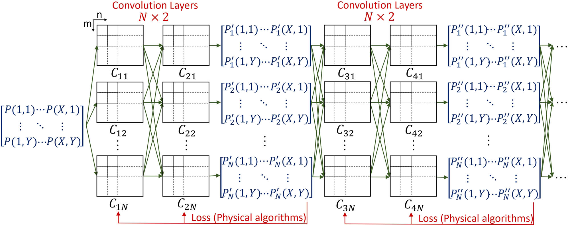
In our approach, Speckle-Net uses multiple unique kernels in each layer as illustrated in Fig. 1. It is worthwhile to emphasize that multiple kernels can produce deep correlations within and between the output objects $P_{i}^{'} (x, y)$ via kernels, where the initial matrices, $P_{i} (x, y)$ , can be either real or complex such as the spatial distribution of intensity and electromagnetic field. The process of constructing deep correlations can be summarized as follows. We employ a total of N kernels $C_{i} (m, n)$ , where $m, n$ are the coordinates of the kernel. The resulting matrices after convolution can be expressed as $P_{i}^{'} (x, y) = \sum_{m, n} C_{i} (m, n) P (x + m, y + n)$ , with $x$ , $y$ being the coordinates of patterns. The ensemble average of patterns is ${\bar{P}}^{'} (x, y) = \sum_{m, n} \bar{C} (m, n) P (x + m, y + n)$ , which actually is an average operation on kernels. Similarly, the fluctuation of each matrix with respect to ${\bar{P}}^{'} (x, y)$ is also working on kernels, $Δ P_{i}^{'} (x, y) = \sum_{m, n} Δ C_{i} (m, n) P (x + m, y + n)$ . Then, the spatial correlation function of the output objects can be expressed as $Γ^{(2)} (Δ x, Δ y) = ⟨ Δ P_{i}^{'} (x_{1}, y_{1}) Δ P_{i}^{'} (x_{2}, y_{2}) ⟩ = ⟨ [\sum_{m_{1}, n_{1}} Δ C_{i} (m_{1}, n_{1}) P (x_{1} + m_{1}, y_{1} + n_{1})] \times [\sum_{m_{2}, n_{2}} Δ C_{i} (m_{2}, n_{2}) P (x_{2} + m_{2}, y_{2} + n_{2})] ⟩ = \sum_{m_{1,2}, n_{1,2}} ⟨ Δ C (m_{1}, n_{1}) Δ C (m_{2}, n_{2}) ⟩ \times P (x_{1} + m_{1}, y_{1} + n_{1}) P (x_{2} + m_{2}, y_{2} + n_{2}) = \sum_{m_{1,2}, n_{1,2}} Γ_{C}^{(2)} (Δ m, Δ n) \times P (x_{1} + m_{1}, y_{1} + n_{1}) P (x_{2} + m_{2}, y_{2} + n_{2}),$ (1)where $Δ x \equiv x_{1} - x_{2}$ , $Δ y \equiv y_{1} - y_{2}$ . In Eq. (1), it is evident that matrices produced by the convolution process exhibit spatial correlations based on the correlation function of the kernel $Γ_{C}^{(2)} (Δ m, Δ n)$ and the initial input matrix. The initial matrices can be considered as weight parameters. Thus, the goal of adjusting kernels in Speckle-Net is to establish deep correlations in the output matrices according to the defined loss function. The convolution of a kernel on a single matrix can be interpreted as a rearrangement of the spatial distribution and statistics of the speckle pattern.

Diagram of Speckle-Net. Speckle-Net consists of multiple branches and two convolution layers within each branch. Subscripts j and i in Cji denote the jth layer and ith kernel in each layer. N kernels are adopted in each layer. A physical algorithm related loss function feedback is applied at the end of each branch to modify the kernels by gradient descent.

Figure 1.Diagram of Speckle-Net. Speckle-Net consists of multiple branches and two convolution layers within each branch. Subscripts $j$ and $i$ in $C_{j i}$ denote the $j$ th layer and $i$ th kernel in each layer. $N$ kernels are adopted in each layer. A physical algorithm related loss function feedback is applied at the end of each branch to modify the kernels by gradient descent.

Apart from kernels, Speckle-Net consists of a multibranch and simplified layer structure compared to traditional neural networks. Single random matrix plays the role of input. A rectifier [39] and a batch normalization [40] are combined into a series of processes after each layer. The rectifier could increase the nonlinearity. The batch normalization is used to avoid covariate shifts between layers so that the $C_{i}$ in each layer should always process data scaled within 0 and 1. Since the speckle pattern is just an intermediate carrier of the experimental process, Speckle-Net has no overfitting issue. Meanwhile, analyzing the matrix and target optical systems through a few intermediate layers is challenging because of the lack of parameters, while too many layers can result in poor directional improvement and increased computational complexity [41]. Thereafter, we choose multibranch architecture [42] to enhance the gradient descent feedback and avoid getting trapped in the local optimum via adjusting parameters in each branch independently. The branch and layer scale can also be adjusted according to the system complexity. For example, the object of the study in the later CGI experiment is correlations between multiple patterns, which needs more parameters than searching phase correlations within one pattern in SIM. Lastly, the evaluations after physical algorithms are flexible. Functions such as mean square error (MSE), contrast-to-noise ratio, and correlation coefficient can be incorporated into the loss function to achieve improved visibility, high contrast, and optimized similarities.

3. IMPLEMENTATION: SUPPRESSING THE CORRELATION FLUCTUATION

A. Application in Computational Ghost Imaging

Ghost imaging [27,43], a single pixel imaging technique, reconstructs the object through the second-order correlation between reference and object light paths. CGI [37,38] substitutes the reference path by preparing speckles in advance. It correlates the collected intensities with illuminating speckle patterns to retrieve images. It has the drawback of a high SR required for the measurement to suppress the correlation fluctuations, which results in a long acquisition time. The SR is defined as $β = N_{s} / N_{p}$ , where $N_{s}$ , $N_{p}$ are the number of sampling patterns and number of pixels in images, respectively. The number of speckle patterns increases immeasurably if the size of the image goes up. Two major directions for improvement have been made. First, techniques such as orthonormalization [32,34] and Fourier and sequential Walsh–Hadamard speckles [44 –46] have been proposed to minimize the SR by carefully designing the speckle arrangement. These algorithm-based techniques improve the overall imaging quality without considering the optimization of each given SR, where the minimum of SRs is around 5%. Besides, compressive sensing [47,48] and deep learning [49 –53] based CGI techniques give much lower SR relying on preknowledge of objects. Nevertheless, these postprocessing techniques and their adaptive objects are limited to the sparsity and categories from the training dataset. Therefore, they will not work or work much worse when objects have a big contradiction to the dataset. In general, CGI is based on a linear aggregation of correlations from each pixel where light passes through. To solve the problem fundamentally and universally, it is natural to be oriented to suppress the second-order correlation fluctuations of the illuminating speckle patterns at low SRs.

We aim to generate deep correlated speckle patterns with minimal correlation variation and optimal speckle size, which can be reflected from the correlation width. To begin with, we include MSE in the loss function of each branch to compare the CGI results with their ground truths. We use the MNIST dataset as the training and part of the testing images. The dataset consists of 60,000 handwritten digits, which have been resized to $112 \times 112$ pixels. Since the backward pass from the loss function only adjusts the kernels, the network should not be limited by the training images, unlike in traditional deep-learning CGI. We trained the network for 200 epochs until the loss stopped declining since overfitting is not an issue in Speckle-Net. This one-time training method gives a group of speckle patterns at any SR, which can then be directly used in the experiment. The images can then be retrieved using the standard CGI algorithm, $Γ^{(2)} (x, y) = ⟨ P (x, y) I ⟩ - ⟨ P (x, y) ⟩ ⟨ I ⟩,$ (2)where $P (x, y)$ are illuminating patterns on DMD, and $I$ are intensities collected by the bucket detector.

We selected four different SRs ( $β = 5 %$ , 2%, 1%, and 0.5%) for Speckle-Net as examples. Once $β$ is set, the number of kernels $N_{k}$ in each layer is determined as $N_{k} = β N_{p} = N_{s}$ . A typical random speckle pattern generated by a $k$ -space aperture [33] is used as the starting pattern. Three training rounds were sufficient to produce optimized patterns for all $β$ values used in this study. In theory, any speckle pattern can be used as the initial input, but the training time varies.

B. Features of the Correlation Fluctuation Suppressed Patterns

Figure 2(a) shows correlated patterns for various $β$ in the left column. It is obvious that the grain size of the speckle pattern gradually decreases when $β$ increases. This feature is also reflected in the Fourier spectrum distribution, which is actually corresponding to the amplitude distribution in $k$ -space. As is presented in the middle column, the frequency component concentrates on low spatial frequencies when $β$ is small and extends to higher spatial frequencies if $β$ increases. It is worth noting that different from the $k$ -space low-pass iris aperture, high-frequency components still exist along the $x = 0$ and $y = 0$ axis in all cases, contributing to the imaging resolution. The most notable advantages of the speckle patterns generated by Speckle-Net are the auto-adjusted correlation width regarding to $β$ and smooth cross correlation at a long correlating distance regardless of $β$ . In the right column of Fig. 2(a), the width of the correlation function becomes narrow when $β = 5 %$ and gradually broadens when $β$ decreases. This feature is automatically given by Speckle-Net, from which we can acquire the optimal solution of correlation width at a specific $β$ . In addition, a spatial visualization of correlations of patterns from Speckle-Net and $k$ -space low-pass aperture is shown in Figs. 2(b) and 2(c), respectively. This suppression of correlation fluctuation distinguishes the deep correlated speckle patterns from traditional incoherent speckle patterns generated by the diffuser plate in which the correlation distribution has a significant random fluctuation due to the lack of enough ensemble average numbers. In Fig. 2(d), we visualize the degree of fluctuation in the 1D section along the dashed line in (a). The correlation of patterns given by Speckle-Net is close to a sinc function and shown to be smooth in the long correlation distance.

Figure 2.(a) Left column: speckle patterns after three-branch Speckle-Net training with $β = 5 %, 2 %, 1 %$ , and 0.5%. Middle column: Fourier spectra of the corresponding patterns (frequency components $f_{x}$ and $f_{y}$ increase from the center to edges). Right column: spatial intensity correlation distributions (correlation distance increases from the center to edges). (b) Spatial correlations of patterns with Speckle-Net and $β = 1 %$ . (c) Spatial correlations ( $β = 1 %$ ) of patterns generated by the diffuser plate. A $k$ -space aperture is applied at the Fourier plane of patterns to control the correlation width the same as in (b). (d) Comparison between two methods with 1D plot along the dashed line marked in (a).

C. Imaging under Low Sampling Ratios

To show the superiority of the deep correlated speckle patterns, we carry out a set of CGI experiments with low SRs. Patterns are programmed onto DMD to illuminate objects. Objects are placed in front of the bucket detector, which collects the transmission light intensity. In the experiments, we used patterns from the three branches of training with SRs of 0.5%, 1%, 2%, and 5% as an example. We adopt four categories of 16 different objects, including simple objects (“three lines,” $π$ , digits “4” and “8”), English letters (“CGI,” “XJTU,” “CITY U,” and “TAMU”), Chinese characters (“xiàng,” “hŭo,” “yán,” and “yàn”), and pictures (“ghost,” “rabbit,” “leaf,” and “Tai Chi”), for reconstruction. In all 16 objects, only digits “4” and “8” are from the pattern training dataset. These objects have different sizes, orientations, and complexities to demonstrate the universal adaptability of deep-learned patterns. CGI with conventional white noise speckle patterns at SR of 5% is also measured for comparison.

The main results are shown in Fig. 3. Simple objects such as the “three lines,” “ $π$ ,” “4,” “8,” and “hŭo” can be reconstructed at only 0.5% SR; i.e., only 62 patterns are used for the illuminating process. At SR of 1%, the basic profile can be reconstructed for most of the objects already, and become much clearer at 2%. At the SR of 5%, all objects can be clearly retrieved. We emphasize that, since patterns possess longer correlation widths under low SRs, images generally show a higher signal-to-background ratio but lower resolution. When the SR goes higher, such as 5%, images have much higher resolution. All of the results illuminated and imaged by the deep correlated speckle patterns keep low background fluctuations. However, in the bottom line, the conventional white noise speckle patterns cannot give any clear imaging results at $β = 5 %$ . In fact, usually white noise CGI cannot be distinguished until the sampling rate reaches 50%. Meanwhile, results sampled from the $k$ -space low-pass filtered pink noise pattern also cannot reach such low fluctuation level [33], which has already been indicated in Figs. 2(b)–2(d). In general, the automatic adapted correlation width and suppressed correlation fluctuation provide the ability to retrieve the object with high resolution and visibility, respectively. This boosts the CGI applicability in extremely low sampling ranges, which might be useful in dynamic imaging systems such as capturing moving objects within a small timescale.

Figure 3.Experimental results of CGI with simple objects (“three lines,” $π$ , digits “4” and “8”), English letters (“CGI,” “XJTU,” “CITY U,” and “TAMU”), Chinese characters (“xiàng,” “hŭo,” “yán,” and “yàn”), and pictures (“ghost,” “rabbit,” “leaf,” and “Tai Chi”) by speckle patterns given from three-branch Speckle-Net. From top to bottom: objects, CGI results with $β = 5 %, 2 %, 1 %, 0.5 %$ with deep correlated patterns, and $β = 5 %$ using conventional white noise patterns, respectively.

To further prove the feasibility, we perform a series of measurements of four objects under different noise levels. We choose the four objects from our four catalogs: the Greek letter “ $π$ ,” the English letter “CGI,” the Chinese character “yán,” and the picture “leaf.” The signal level is scaled by the signal-to-noise ratio (SNR) value defined as $SNR = 10 \log (P_{s} / P_{b})$ , where $P_{s}$ is the average intensity in each signal pixel and $P_{b}$ is the average intensity in the noise background. Here we choose three different SNR conditions: 88 dB, 6.4 dB, and 3.1 dB. In Fig. 4, it is clearly seen that at 8.8 dB, all the images can be retrieved regardless of SRs. When the SNR is 6.4 dB, some images start to show the noisy background. Nevertheless, all the objects can still be clearly identified. At the noisy condition, with SNR being 3.1 dB, most of the objects can still be identified. We also notice that speckle patterns with lower SR are more robust to noise interference since they are illuminated by patterns with a lower frequency spectrum. High-frequency noises are automatically filtered out during the sampling process. Take the Greek letter “ $π$ ” for example; although it can be clearly imaged at 3.1 dB when the SR is 5%, noticeable background noise exists in the resulting image. At 2% SR, the background noise starts to degrade. When the SR is at 1% or 0.5%, the background is almost smooth, and we see nearly no difference between the results at three levels.

Figure 4.Experimental results of CGI using deep correlated speckles with various noise levels labeled in the left column. (a) $β = 5 %$ , (b) $β = 2 %$ , (c) $β = 1 %$ , and (d) $β = 0.5 %$ .

4. IMPLEMENTATION: SUPPRESSING THE OPTICAL DIFFRACTION

A. Application in Structured Illumination Microscopy

The statistics and diffraction of the beam profile are also valuable research aspects for various applications, such as structured illumination imaging and sensing [11,13,54,55]. Compared to the commonly used Rayleigh speckle, super-Rayleigh and other types of customized speckles can improve high-order correlation-based imaging and microscopy qualities [25,26,56,57]. Typically, by carefully designing the intensity statistics of speckles used in parallelized nonlinear pattern-illumination microscopy, it enables us to retrieve a three-times higher spatial resolution than the optical diffraction limit [25]. Nevertheless, the diffraction effect restricts the above customized non-Rayleigh speckles from exploiting their advantages from the axial direction. In other words, SIM cannot always keep the high-resolution tomography or 3D microscopy with long distance [23,58]. In detail, a laser beam initially confined to a finite area in a transverse plane will be subject to diffractive spreading as it propagates outward from that plane in a free space. The intensity profile of speckle patterns varies as the beam propagates. There is always a trend for speckles to follow the standard Rayleigh distribution no matter what distribution it originally began with. For instance, the standard Rayleigh speckles keep their distribution and contrast, while other non-Rayleigh speckles rapidly fall back to the standard Rayleigh distribution only in a small Rayleigh range, which corresponds to the transverse length of a single speckle. Conclusively, various schemes have been proposed to generate non-Rayleigh statistics speckles [23,25,26,30,59,60], some works proposed methods for generating nondiffracting speckle patterns [61 –63], and a few works tried to get both features at the same time [22,64]. Particularly, it has been proposed to generate NRND speckle patterns via using a ring-shape aperture together with asymmetric phase modulation at the Fourier plane of the speckle pattern [22]. The non-Rayleigh statistics can last for $20 R$ with much slower decay rate compared to the traditional non-Rayleigh speckle patterns. However, this nondiffracting effect is created based on the ring-shape apertures, where an optical power attenuation occurs when light passes through the aperture. In several applications, high optical power is urgently needed. For instance, in the ultracold atomic quantum simulations, strong disorder strength requires high optical power to provide strong enough dipole force [21] since the disorder sources are usually picked at far detuning to suppress the scattering effect.

We conceive that it will be useful if Speckle-Net can provide us with a group of phase masks that can generate NRND patterns without any amplitude modulation. The advantage is that by performing phase modulation, the optical power only gets spatially redistributed but remains conservative in total. To begin with, we first set a random phase mask with $500 \times 500$ pixels in Speckle-Net. After convoluting with several layers of kernels, a new phase mask $ϕ (f_{x}, f_{y})$ will be provided. Then at the phase modulation plane, in theory, the Fourier spectrum can be interpreted as $g (f_{x}, f_{y}) = A (f_{x}, f_{y}) e^{i ϕ (f_{x}, f_{y})}$ , where $A (f_{x}, f_{y})$ represents the amplitude of the Fourier spectrum. Since we only intend to do the phase modulation in the experiment, we set $A (f_{x}, f_{y}) \equiv 1$ by default. Thereafter, the intensity distribution of the speckle pattern with propagation distance $z$ from the initial position can be expressed as $I (x, y, z) = | E (x, y, z {) |}^{2} \propto | I F {g (f_{x}, f_{y})} H (f_{x}, f_{y}, z {) |}^{2},$ (3)where $I F {}$ is the notation for the inverse Fourier transform, and $E (x, y, z)$ is the interpretation for the light field. The Fourier convolution theorem is applied, and here $H (f_{x}, f_{y}, z)$ is the Rayleigh–Sommerfeld transfer function [65] given by $H (f_{x}, f_{y}, z) = \exp [i k z \sqrt{1 - {(λ f_{x})}^{2} - {(λ f_{y})}^{2}}]$ . Here, $λ$ is the optical wavelength; $k$ is the wavenumber, which is equal to $2 π / λ$ for free space; and $z$ is the distance between the initial position and observation coordinate position. The Rayleigh range is set as a unit for distance $z$ in the simulation and experiment. In the end, we define the spatial statistics of speckle patterns by looking at the contrast. The expression of the contrast $C$ is $C (z) = \frac{\sqrt{Var (I (x, y, z))}}{\bar{I (x, y, z)}},$ (4)where $\bar{I}$ is the average intensity of pixels in the transverse plane, and $Var (\cdot)$ is the variance operator. We select propagation distance within 60 Rayleigh ranges. The contrast at every one Rayleigh range is calculated to obtain an array of contrast $C (z)$ of speckle patterns during light propagation. The Speckle-Net’s loss function is thereafter defined as the inverse of averaged contrast $\bar{C (z)}$ , which means when the loss function turns to converge to 0, the averaged contrast $\bar{C (z)}$ increases. As mentioned in the CGI part, the overfitting effect is not an issue, so we set the network training for 200 epochs where the loss stops declining. The first branch already gives NRND speckle patterns, so we drop the following branches. Overall, the training of Speckle-Net provides us with a well-trained phase mask that could generate NRND speckle patterns.

B. Features of the Nondiffracting Non-Rayleigh Patterns

Similarly, to reveal the generation mechanism of the NRND speckle pattern, we choose a group of phase masks and perform the spatial correlation between pixels in the mask. Rather than the noncorrelated random phases, it indicates distinctive spatial correlations as is shown in Fig. 5. What we can learn from the Speckle-Net is that the existence of negative values in a long propagation distance shown in the neighborhood cross correlations explains the reason for the nondiffracting effect for non-Rayleigh speckles. The anti-correlated phases close to each other tend to give destructive interference on the objective plane, therefore giving large dark areas and sparse speckles. In Fig. 5(a), each phase is correlated with its diagonal pixels and anti-correlated with its near-neighborhood pixels. After $7.5 R$ propagation, the anti-correlated pixels shift to further distance while the correlation strength is still lower than $- 0.2$ [Fig. 5(b)]. When the super-Rayleigh returns back to standard Rayleigh speckles at $z = 15 R$ in Fig. 5(c), the correlation strength of the anti-correlated pixels tends to be 0, and the number of correlated/anti-correlated pixels substantially decreases. In Fig. 5(d) we present the phase correlation of $z = 45 R$ , and it becomes almost random noncorrelated, which follows the feature of standard Rayleigh speckle patterns.

Figure 5.Spatial correlation of phase masks at the Fourier plane of (a) $z = 0 R$ , (b) $z = 7.5 R$ , (c) $z = 15 R$ , and (d) $z = 45 R$ . The result is ensemble averaged 10,000 times.

Apart from the phase spatial correlation, we also check the non-Rayleigh characteristics by searching nonlocal correlations of electromagnetic field, $Γ_{4}^{(2)}$ . By picking up the speckle pattern at the peak contrast ( $z = 7.5 R$ ), we perform the inverse Fourier transform and obtain its Fourier intensity spectrum. We extract the amplitude by applying the square root. Along with the phase information, then, we obtain the $Γ_{4}^{(2)}$ of the electromagnetic field. It follows the nonlocal second-order correlation algorithm [30]. For reference, the standard Rayleigh speckle pattern’s $Γ_{4}^{(2)}$ is calculated as well. With 10,000 ensemble time, $Γ_{4}^{(2)}$ is $\sim 15$ for the non-Rayleigh speckle pattern, and $\sim 0.13$ for the standard Rayleigh speckle pattern.

C. Measurements on the Degree of Diffraction and Intensity Statistics

To verify the robustness of optical diffraction, we load phase masks onto SLM in SIM. In detail, a nearly perfect 532 nm collimated beam cleaned by a single-mode fiber is shined onto a phase-only SLM, where the $500 \times 500$ pixels deep correlated phase mask is loaded. One lens performs an inverse Fourier transform and focuses the speckle pattern to the microscope objective plane ( $z = 0$ plane at the beam waist). The overall procedure does not cost any optical power loss except for mechanical defects. A CCD takes images along the axial axis within $45 R$ with $δ z = 2.5 R$ per step. To a good approximation, the field incident on the camera (at $z = 0 R$ ) is an inverse Fourier transform of the field reflected off the SLM. This process is repeated eight times to obtain the averaged contrasts and measurement errors at each plane, shown in Fig. 6(b). In Fig. 6(a), we pick one image of the speckle pattern of each plane as an example. The width of the radial correlation function of speckle intensity is around 20 μm; then the Rayleigh range is 2.3 mm. After we modulate the laser field, the interference pattern evolves upon axial propagation and gradually turns from sub-Rayleigh to super-Rayleigh distribution. After $7.5 R$ , the contrast increases to the maximum, $C = 1.60$ . Intuitively, Fig. 6(a) indicates that the speckles at $z = 7.5 R$ are more concentrated and sparser than speckles taken from other positions. The contrast of the speckle pattern can keep above $\sqrt{2}$ within four Rayleigh ranges, and then slowly drop to $C \sim 1.03$ at $z = 22.5 R$ . It revives toward $C \sim 1.12$ speckles again at $z = 27.5 R$ , and the contrast remains more than 1.1 for another $12.5 R$ before $40 R$ . In addition, we also plot the statistics of the PDF, $P (I, z)$ , based on various propagation distances. In a logarithmic plot, the standard Rayleigh distribution should roughly obey the straight line, while the sub-Rayleigh and super-Rayleigh ought to be convex and concave curvatures, respectively. In Fig. 7, the PDF of the speckle pattern at $z = 0 R$ follows the sub-Rayleigh distribution since its $P (I \sim 0, z = 0 R)$ is below the straight dashed line while $P (I \sim 256, z = 0 R)$ is above, which indicates that its contrast is slightly lower than 1. After $7.5 R$ propagation, the PDF curve tends to be convex because both low and high intensity pixel numbers increase. Thereafter, in Fig. 6(b) the contrast improves, reaches a maximum at $z = 7.5 R$ , and slowly declines to 1. The later-on speckle patterns after $z = 22.5 R$ remain with the contrast around 1.1, and their intensities follow a super-Rayleigh distribution. For comparison, we also simulate the traditional well-established situations in which the random and central asymmetrical phase distributions with exactly the same field distribution are loaded at the Fourier plane. The random phase distribution provides the standard Rayleigh speckle patterns whose contrast remains around 1, while the central asymmetrical phase distribution presents the super-Rayleigh distribution only within $2.5 R$ . The decay rate is much faster than the speckle patterns modulated from the phase masks given by the Speckle-Net. Overall, considering the real environmental noise and hardware defects, we are able to achieve a continuous super-Rayleigh speckle pattern in $Δ z \sim 20 R$ , and it revives to super-Rayleigh afterwards.

Figure 6.Experimental results from the structured illumination microscope with deep correlated phase masks. (a) Speckle patterns captured by CCD with various propagation distances. (b) Contrast of speckle patterns corresponding to the propagation distance. The red dots are measurements of contrast of speckle patterns given by Speckle-Net phase masks, where each data point is repeated eight times with an errorbar. The solid blue line represents the contrast of super-Rayleigh speckle patterns starting with asymmetric random phase. The black dashed line shows the contrast of standard Rayleigh speckle patterns without the phase mask. Dashed gray line is a reference for $C = 1$ .

Figure 7.Probability density function in transverse planes. $P (I)$ is the probability of intensity I ( $0 - 255$ ) in its corresponding transverse plane. The dashed lines are seated on $z = 0 R$ , $z = 7.5 R$ , and $z = 45 R$ .

5. CONCLUSION AND DISCUSSION

In summary, we propose a “catch all” scheme through the use of machine learning concepts and physics algorithms to encode features in patterns. We select the CGI and SIM as our objectives and aim at high CGI sampling efficiency and suppressed diffraction in non-Rayleigh patterns, respectively. We verify that the Speckle-Net can provide us with deep correlations in intensity and phase regime. Neither optimized suppression of correlation fluctuation nor long-lasting anti-correlating phases have ever been explored and can be an instruction to solve problems in CGI and SIM fundamentally. Experimentally, we demonstrate that the speckle patterns do have the ability to enhance imaging efficiency and be robust to noise in CGI. This method is unique and superior to traditional CGI and deep-learning-based CGI from the aspect of imaging quality and category. Besides, we also prove that it owns an ability to generate non-Rayleigh speckle patterns that can propagate long distances with a low diffracting rate of the intensity statistics. The Speckle-Net encodes a unique phase mask toward the light field whose deep correlation can be held for continuous $\sim 20 R$ . In addition, we believe that other structures together with kernels, such as U-net [66] and recurrent neural network (RNN) [67], can also be explored and modified similarly to generate aimed speckle patterns. As an example, the time-dependent RNN can be modified similarly in order to create time-dependent patterns, according to the instant feedback and demand of systems.

References

[1] D. J. Pine, D. A. Weitz, P. M. Chaikin. Diffusing wave spectroscopy. Phys. Rev. Lett., 60, 1134-1137(1988).

[2] S.-W. Li, F. Li, T. Peng. Photon statistics of quantum light on scattering from rotating ground glass. Phys. Rev. A, 101, 063806(2020).

[3] J. W. Goodman. Statistical properties of laser speckle patterns. Laser Speckle and Related Phenomena, 9-75(1975).

[4] I. Zanette, T. Zhou, A. Burvall. Speckle-based X-ray phase-contrast and dark-field imaging with a laboratory source. Phys. Rev. Lett., 112, 253903(2014).

[5] J. Wang, A. Z. Genack. Transport through modes in random media. Nature, 471, 345-348(2011).

[6] L. Olivieri, J. S. T. Gongora, L. Peters. Hyperspectral terahertz microscopy via nonlinear ghost imaging. Optica, 7, 186-191(2020).

[7] G. C. Valley, G. A. Sefler, T. J. Shaw. Multimode waveguide speckle patterns for compressive sensing. Opt. Lett., 41, 2529-2532(2016).

[8] B. Redding, S. M. Popoff, H. Cao. All-fiber spectrometer based on speckle pattern reconstruction. Opt. Express, 21, 6584-6600(2013).

[9] T. Strudley, T. Zehender, C. Blejean. Mesoscopic light transport by very strong collective multiple scattering in nanowire mats. Nat. Photonics, 7, 413-418(2013).

[10] B. Redding, S. F. Liew, R. Sarma. Compact spectrometer based on a disordered photonic chip. Nat. Photonics, 7, 746-751(2013).

[11] C. Ventalon, J. Mertz. Dynamic speckle illumination microscopy with translated versus randomized speckle patterns. Opt. Express, 14, 7198-7209(2006).

[12] J. Mertz. Optical sectioning microscopy with planar or structured illumination. Nat. Methods, 8, 811-819(2011).

[13] E. Mudry, K. Belkebir, J. Girard. Structured illumination microscopy using unknown speckle patterns. Nat. Photonics, 6, 312-315(2012).

[14] S. Nakadate, H. Saito. Fringe scanning speckle-pattern interferometry. Appl. Opt., 24, 2172-2180(1985).

[15] H. Yilmaz, E. G. van Putten, J. Bertolotti. Speckle correlation resolution enhancement of wide-field fluorescence imaging. Optica, 2, 424-429(2015).

[16] M. Pascucci, G. Tessier, V. Emiliani. Superresolution imaging of optical vortices in a speckle pattern. Phys. Rev. Lett., 116, 093904(2016).

[17] V. Doya, O. Legrand, F. Mortessagne. Speckle statistics in a chaotic multimode fiber. Phys. Rev. E, 65, 056223(2002).

[18] J. Wang, S. K. Nadkarni. The influence of optical fiber bundle parameters on the transmission of laser speckle patterns. Opt. Express, 22, 8908-8918(2014).

[19] W. McGehee, S. Kondov, W. Xu. Three-dimensional Anderson localization in variable scale disorder. Phys. Rev. Lett., 111, 145303(2013).

[20] D. Delande, G. Orso. Mobility edge for cold atoms in laser speckle potentials. Phys. Rev. Lett., 113, 060601(2014).

[21] E. Fratini, S. Pilati. Anderson localization of matter waves in quantum-chaos theory. Phys. Rev. A, 91, 061601(2015).

[22] R. Liu, B. Qing, S. Zhao. Generation of non-Rayleigh nondiffracting speckles. Phys. Rev. Lett., 127, 180601(2021).

[23] S. Han, N. Bender, H. Cao. Tailoring 3D speckle statistics. Phys. Rev. Lett., 130, 093802(2023).

[24] M. Saxena, G. Eluru, S. S. Gorthi. Structured illumination microscopy. Adv. Opt. Photonics, 7, 241-275(2015).

[25] N. Bender, M. Sun, H. Ylmaz. Circumventing the optical diffraction limit with customized speckles. Optica, 8, 122-129(2021).

[26] Z. Li, X. Nie, F. Yang. Sub-Rayleigh second-order correlation imaging using spatially distributive colored noise speckle patterns. Opt. Express, 29, 19621-19630(2021).

[27] R. S. Bennink, S. J. Bentley, R. W. Boyd. “two-photon” coincidence imaging with a classical source. Phys. Rev. Lett., 89, 113601(2002).

[28] X.-H. Chen, Q. Liu, K.-H. Luo. Lensless ghost imaging with true thermal light. Opt. Lett., 34, 695-697(2009).

[29] A. Valencia, G. Scarcelli, M. D’Angelo. Two-photon imaging with thermal light. Phys. Rev. Lett., 94, 063601(2005).

[30] Y. Bromberg, H. Cao. Generating non-Rayleigh speckles with tailored intensity statistics. Phys. Rev. Lett., 112, 213904(2014).

[31] H. E. Kondakci, A. Szameit, A. F. Abouraddy. Sub-thermal to super-thermal light statistics from a disordered lattice via deterministic control of excitation symmetry. Optica, 3, 477-482(2016).

[32] B. Luo, P. Yin, L. Yin. Orthonormalization method in ghost imaging. Opt. Express, 26, 23093-23106(2018).

[33] X. Nie, F. Yang, X. Liu. Noise-robust computational ghost imaging with pink noise speckle patterns. Phys. Rev. A, 104, 013513(2021).

[34] X. Nie, X. Zhao, T. Peng. Sub-Nyquist computational ghost imaging with orthonormal spectrum-encoded speckle patterns. Phys. Rev. A, 105, 043525(2022).

[35] K. Fukushima. Neocognitron: a self-organizing neural network model for a mechanism of pattern recognition unaffected by shift in position. Biol. Cybern., 36, 193-202(1980).

[36] A. Krizhevsky, I. Sutskever, G. E. Hinton. Imagenet classification with deep convolutional neural networks. Commun. ACM, 60, 84-90(2017).

[37] J. H. Shapiro. Computational ghost imaging. Phys. Rev. A, 78, 061802(2008).

[38] Y. Bromberg, O. Katz, Y. Silberberg. Ghost imaging with a single detector. Phys. Rev. A, 79, 053840(2009).

[39] V. Nair, G. E. Hinton. Rectified linear units improve restricted Boltzmann machines. International Conference on Machine Learning, 807-814(2010).

[40] S. Ioffe, C. Szegedy. Batch normalization: Accelerating deep network training by reducing internal covariate shift. International Conference on Machine Learning, 448-456(2015).

[41] K. He, X. Zhang, S. Ren. Identity mappings in deep residual networks. European Conference on Computer Vision, 630-645(2016).

[42] X. Zhu, M. Bain. B-CNN: branch convolutional neural network for hierarchical classification. arXiv(2017).

[43] T. B. Pittman, Y. Shih, D. Strekalov. Optical imaging by means of two-photon quantum entanglement. Phys. Rev. A, 52, R3429-R3432(1995).

[44] L. Wang, S. Zhao. Fast reconstructed and high-quality ghost imaging with fast Walsh–Hadamard transform. Photonics Res., 4, 240-244(2016).

[45] Z. Zhang, X. Ma, J. Zhong. Single-pixel imaging by means of Fourier spectrum acquisition. Nat. Commun., 6, 6225(2015).

[46] Z. Zhang, X. Wang, G. Zheng. Hadamard single-pixel imaging versus Fourier single-pixel imaging. Opt. Express, 25, 19619-19639(2017).

[47] O. Katz, Y. Bromberg, Y. Silberberg. Compressive ghost imaging. Appl. Phys. Lett., 95, 131110(2009).

[48] V. Katkovnik, J. Astola. Compressive sensing computational ghost imaging. J. Opt. Soc. Am. A, 29, 1556-1567(2012).

[49] M. Lyu, W. Wang, H. Wang. Deep-learning-based ghost imaging. Sci. Rep., 7, 17865(2017).

[50] T. Shimobaba, Y. Endo, T. Nishitsuji. Computational ghost imaging using deep learning. Opt. Commun., 413, 147-151(2018).

[51] G. Barbastathis, A. Ozcan, G. Situ. On the use of deep learning for computational imaging. Optica, 6, 921-943(2019).

[52] F. Wang, H. Wang, H. Wang. Learning from simulation: an end-to-end deep-learning approach for computational ghost imaging. Opt. Express, 27, 25560-25572(2019).

[53] H. Wu, R. Wang, G. Zhao. Sub-Nyquist computational ghost imaging with deep learning. Opt. Express, 28, 3846-3853(2020).

[54] D. Lim, K. K. Chu, J. Mertz. Wide-field fluorescence sectioning with hybrid speckle and uniform-illumination microscopy. Opt. Lett., 33, 1819-1821(2008).

[55] A. Vigoren, J. M. Zavislan. Optical sectioning enhancement using higher-order moment signals in random speckle-structured illumination microscopy. J. Opt. Soc. Am. A, 35, 474-479(2018).

[56] K. Kuplicki, K. W. C. Chan. High-order ghost imaging using non-Rayleigh speckle sources. Opt. Express, 24, 26766-26776(2016).

[57] P. Liu. Label-free storm principle realized by super-Rayleigh speckle in photoacoustic imaging. Opt. Lett., 44, 4642-4645(2019).

[58] M. Pascucci, S. Ganesan, A. Tripathi. Compressive three-dimensional super-resolution microscopy with speckle-saturated fluorescence excitation. Nat. Commun., 10, 1327(2019).

[59] N. Bender, H. Ylmaz, Y. Bromberg. Customizing speckle intensity statistics. Optica, 5, 595-600(2018).

[60] N. Bender, H. Ylmaz, Y. Bromberg. Creating and controlling complex light. APL Photonics, 4, 110806(2019).

[61] J. Durnin. Exact solutions for nondiffracting beams. I. The scalar theory. J. Opt. Soc. Am. A, 4, 651-654(1987).

[62] A. Vasara, J. Turunen, A. T. Friberg. Realization of general nondiffracting beams with computer-generated holograms. J. Opt. Soc. Am. A, 6, 1748-1754(1989).

[63] L. Vicari. Truncation of non diffracting beams. Opt. Commun., 70, 263-266(1989).

[64] J. G. Neto, E. J. Fonseca, A. J. Jesus-Silva. Exact solutions for non-Rayleigh nondiffracting speckles. Phys. Rev. A, 106, 053519(2022).

[65] D. G. Voelz. Computational Fourier Optics: A MATLAB Tutorial, 534(2011).

[66] O. Ronneberger, P. Fischer, T. Brox. U-net: convolutional networks for biomedical image segmentation. International Conference on Medical Image Computing and Computer-Assisted Intervention, 234-241(2015).

[67] J. T. Connor, R. D. Martin, L. E. Atlas. Recurrent neural networks and robust time series prediction. IEEE Trans. Neural Netw., 5, 240-254(1994).