Researching | Deep plug-and-play priors for spectral snapshot compressive imaging

Journals >Photonics Research >Volume 9 >Issue 2 >Page B18 > Article

Photonics Research
Vol. 9, Issue 2, B18 (2021)

Deep plug-and-play priors for spectral snapshot compressive imaging

Siming Zheng^1、2、†, Yang Liu^3、†, Ziyi Meng⁴, Mu Qiao⁵, Zhishen Tong^6、7, Xiaoyu Yang^1、2, Shensheng Han^6、7, and Xin Yuan^8、*

Author Affiliations

¹Computer Network Information Center, Chinese Academy of Sciences, Beijing 100190, China

²University of Chinese Academy of Sciences, Beijing 100049, China

³Computer Science and Artificial Intelligence Laboratory, Massachusetts Institute of Technology, Cambridge, Massachusetts 02139, USA

⁴Beijing University of Posts and Telecommunications, Beijing 100876, China

⁵New Jersey Institute of Technology, Newark, New Jersey 07102, USA

⁶Key Laboratory for Quantum Optics and Center for Cold Atom Physics of CAS, Shanghai Institute of Optics and Fine Mechanics, Chinese Academy of Sciences, Shanghai 201800, China

⁷Center of Materials Science and Optoelectronics Engineering, University of Chinese Academy of Sciences, Beijing 100049, China

⁸Nokia Bell Labs, Murray Hill, New Jersey 07974, USA

show less

DOI: 10.1364/PRJ.411745 Cite this Article Set citation alerts

Siming Zheng, Yang Liu, Ziyi Meng, Mu Qiao, Zhishen Tong, Xiaoyu Yang, Shensheng Han, Xin Yuan. Deep plug-and-play priors for spectral snapshot compressive imaging[J]. Photonics Research, 2021, 9(2): B18 Copy Citation Text

show less

Generalized image formation (left) and the discrete matrix-form model (right) of spectral SCI. Here color denotes the corresponding spectral band.

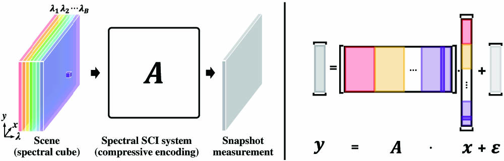
Fig. 1. Generalized image formation (left) and the discrete matrix-form model (right) of spectral SCI. Here color denotes the corresponding spectral band.

Download full size | View in the Article

Comparison of image-plane coding (upper) and aperture-plane coding (lower) spectral SCI systems in terms of sensing matrix. Here each color block denotes the corresponding transport matrix at that spectral band.

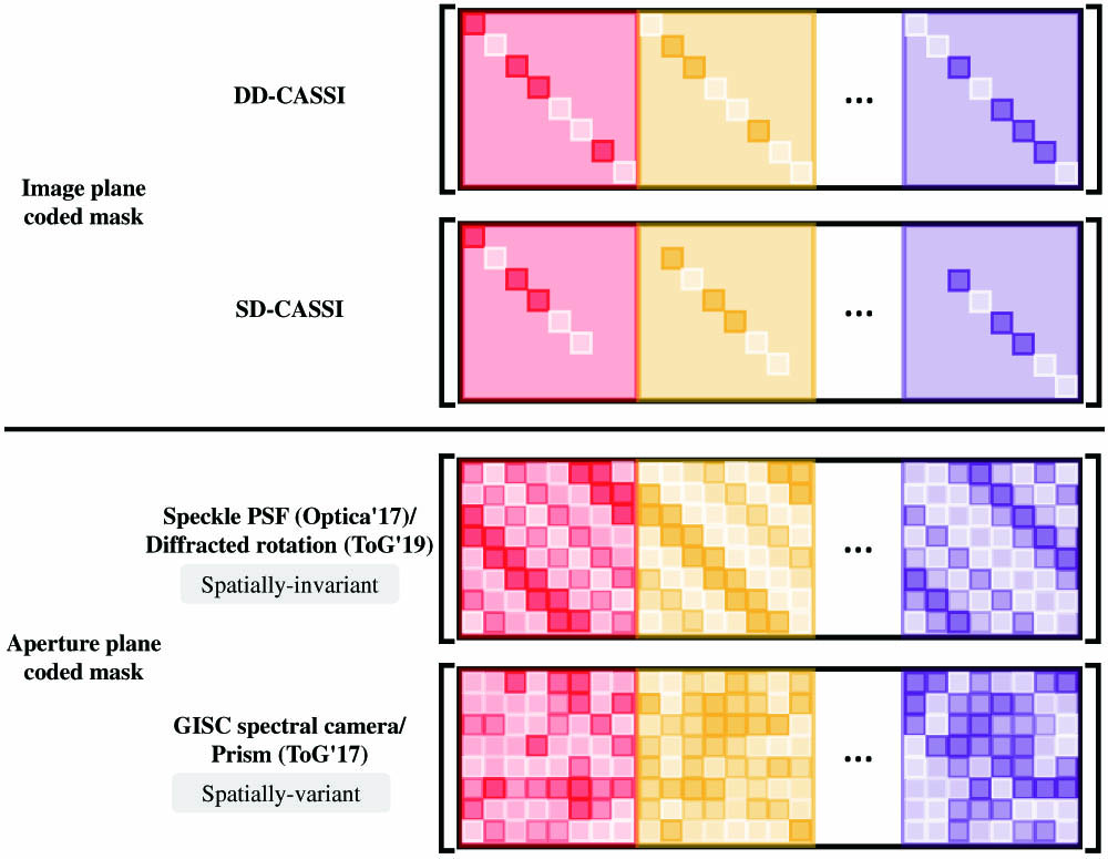
Fig. 2. Comparison of image-plane coding (upper) and aperture-plane coding (lower) spectral SCI systems in terms of sensing matrix. Here each color block denotes the corresponding transport matrix at that spectral band.

Download full size | View in the Article

Fig. 3. Image formation process of a typical spectral SCI system, i.e., SD-CASSI and the reconstruction process using the proposed deep PnP prior algorithm.

Download full size | View in the Article

Fig. 4. Network structure of the deep spectral denoising prior.

Download full size | View in the Article

Fig. 5. Test spectral data from (a) ICVL [69] and (b) KAIST [35] data sets used in simulation. The reference RGB images with pixel resolution 256×256 are shown here. We crop similar regions of the whole image for spatial sizes of 512×512 and 1024×1024.

Download full size | View in the Article

Fig. 6. Simulation results of color-checker with size of 256×256 from KAIST data set compared with the ground truth. PSNR and SSIM results are also shown for each algorithm.

Download full size | View in the Article

Fig. 7. Simulation results of exemplar scenes (top, ICVL; bottom, KAIST) with size of 256×256 compared with the ground truth. Spectral curves of selected regions are also plotted to compare with the ground truth.

Download full size | View in the Article

Fig. 8. Simulation results of four selected scenes shown in sRGB and spectral curves with spatial size of 512×512 (shown in full size in the far left column). The spectra of the pinned (yellow) region of the close-up are shown on the right.

Download full size | View in the Article

Fig. 9. Simulation results of four selected scenes shown in sRGB and spectral curves with spatial size of 1024×1024 (shown in full size in the far left column). The spectra of the pinned (yellow) region of the close-up are shown on the right.

Download full size | View in the Article

Fig. 10. Real data, object SD-CASSI data (256×210×33).

Download full size | View in the Article

Fig. 11. Real data, bird SD-CASSI data (1021×731×33).

Download full size | View in the Article

Fig. 12. Real data, Lego SD-CASSI data (660×550×28).

Download full size | View in the Article

Fig. 13. Real data, plant SD-CASSI data (660×550×28).

Download full size | View in the Article

Fig. 14. Real data, snapshot multispectral endomicroscopy data (660×660×24).

Download full size | View in the Article

Fig. 15. Real data, GISC spectral camera data (330×330×16).

Download full size | View in the Article

Spatial Size	Data Set	TwIST			GAP-TV			AE			U-net			PnP
Spatial Size	Data Set	PSNR (dB)	SSIM	Running Time (s)	PSNR (dB)	SSIM	Running Time (s)	PSNR (dB)	SSIM	Running Time (s)	PSNR (dB)	SSIM	Running Time (s)	PSNR (dB)	SSIM	Running Time (s)
$256 \times 256$	ICVL	30.58	0.8731	156.3	32.57	0.8794	130.2	29.41	0.8711	144.2	31.13	0.8897	0.8	35.03	0.9274	132.7
$256 \times 256$	KAIST	27.32	0.8495	156.3	29.66	0.8584	130.2	26.79	0.8498	144.2	29.44	0.8941	0.8	33.21	0.9273	132.7
$512 \times 512$	ICVL	31.82	0.8955	1380.2	33.58	0.8965	399.1	31.22	0.8969	493.6	NA	NA	NA	35.68	0.9319	401.6
$512 \times 512$	KAIST	29.09	0.8944	1380.2	31.38	0.8993	399.1	29.28	0.8974	493.6	NA	NA	NA	34.29	0.9378	401.6
$1024 \times 1024$	ICVL	32.68	0.9159	3657.6	34.22	0.9157	1460.7	32.03	0.9158	2053.5	NA	NA	NA	36.21	0.9434	1453.6
$1024 \times 1024$	KAIST	31.64	0.9099	3657.6	33.66	0.9134	1460.7	31.05	0.9071	2053.5	NA	NA	NA	36.41	0.9433	1453.6

Table 1. Average PSNR (in dB), SSIM, and Running Time (in Seconds) of 16 Simulation Scenes (8 from ICVL and 8 from KAIST) at Different Spatial Sizes Using Various Algorithms^a

View in the Article

Figures&Tables (16)

References (72)

Copy Citation Text

Siming Zheng, Yang Liu, Ziyi Meng, Mu Qiao, Zhishen Tong, Xiaoyu Yang, Shensheng Han, Xin Yuan. Deep plug-and-play priors for spectral snapshot compressive imaging[J]. Photonics Research, 2021, 9(2): B18

Download Citation

Set citation alerts for the article

Set citation alerts for the article

Save the article for my favorites

Paper Information

Recommended Topics

laser devices and laser physics

Lasers and Laser Optics

laser manufacturing

Instrumentation, Measurement and Metrology

Set citation alerts for the article

Please enter your email address