Real scenes are spectrally rich. Capturing the color, and thus the spectral information, has been a central issue since the dawn of photography. Correspondingly, many strategies have been considered. Since the advent of solid-state imaging, the color filter array and especially the red–green–blue (RGB) bayer filter have been the dominant strategy [1]. These filter arrays usually only capture red, green, and blue bands and thus limit the spectral resolution. When the number of sampled wavelengths becomes large, bandpass filters, push-room, and other strategies may be desirable. These systems usually have limited temporal resolution due to the inherent scanning procedure. Advances in photonics and 2D materials give rise to compact solutions to single-shot spectrometers at a high spectral resolution [2–5]. More recently, it has been applied for spectral imaging via combining stacking [6], optical parallelization [7], and compressive sampling [8] strategies, where the trade-off between the spatial pixel and spectral resolution still remains a challenge. Thanks to compressive sensing (CS) [9–11] and the advent of decompressive inference algorithms over the past couple of decades, there is substantial interest in hyperspectral color filter arrays [12–14]. Such sampling strategies capture localized coded image features and are well-matched to sparsity-based inference algorithms [15–17]. With these advanced algorithms, this technique has led to single-shot imaging for hyperspectral images (HSIs), and we dub it snapshot compressive imaging (SCI) [16,18]. In this paper, we focus on the spectral SCI, which aims to measure the $(x,y,\lambda )$ data cube.

Spectral SCI is a hardware encoder plus software decoder system, where the hardware encoder denotes the optical system, which compresses the 3D $(x,y,\lambda )$ data cube to a snapshot measurement on the 2D detector, and the software decoder denotes the reconstruction algorithms used to recover the 3D data cube from the snapshot measurement.

The underlying principle of the spectral SCI hardware is to modulate different bands (corresponding to different wavelengths) in the spectral data cube by different weights and then integrate the light to the sensor. To perform the modulation, which should be different for different spectral bands, various techniques have been used. The pioneer work of coded aperture snapshot spectral imaging (CASSI) [12] used a fixed mask (coded aperture) and two dispersers to implement the band-wise modulation, termed DD-CASSI; here DD means dual disperser. Following this, the single-disperser (SD) CASSI was developed [19], which achieves modulation by removing a disperser. Following CASSI, various spectral SCI systems have been built using disperser/prism and masks [20–24]. Recently, motivated by the spectral variant responses of other media, spatial light modulators [25], ground-glass-based light field modulation [26], and scatters [27] have also been employed for spectral SCI. In addition, some compact systems have also been built [28,29].

The software decoder, i.e., the reconstruction algorithm, plays a pivotal role in spectral SCI as it outputs the desired data cube. At the beginning, optimization-based algorithms developed for inverse problems such as CS were employed. Since spectral SCI is an ill-posed problem, regularizers or priors are generally used, such as the sparsity [30] and total variation [15]. Later, the patch-based methods such as dictionary learning [25,31] and Gaussian mixture models [32] were developed for the reconstruction of spectral SCI. Recently, by utilizing the nonlocal similarity in the spectral data cube, group sparsity [17] and low-rank models [16] have been developed to achieve state-of-the-art results. The main bottleneck of these high performance iterative optimization-based algorithms is the low reconstruction speed. Since the spectral data cube is usually large-scale, sometimes it needs hours to reconstruct a spectral data cube from a snapshot measurement. This precludes the real applications of spectral SCI systems.

To address the above speed issue in optimization algorithms, and inspired by the performance of deep-learning approaches for other inverse problems [33,34], convolutional neural networks (CNNs) have been used to solve the inverse problem of spectral SCI for the sake of high speed [35–39]. These networks have led to better results than their optimization counterparts, given sufficient training data and time, which usually take days or weeks. After training, the network can output the reconstruction instantaneously and thus lead to end-to-end spectral SCI sampling and reconstruction [39]. However, these networks are usually system-specific. For example, different numbers of spectral bands exist in different spectral SCI systems. Further, due to the different designs of masks, the trained CNNs cannot be used in other systems, while retraining a new network from scratch would take a long time.

Bearing the above concerns in mind, i.e., optimization-based and deep-learning-based algorithms each have their own pros and cons, it is desirable to develop a fast, flexible, and high accuracy algorithm for spectral SCI. Fortunately, the plug-and-play (PnP) framework [40,41] has been proposed for inverse problems with provable convergence [42,43]. The idea of PnP is intuitive, since the goal is to use the state-of-the-art denoiser as a simple plug-in for recovery. The rationale here is to employ recent advanced deep denoisers [44–46] in the iterative optimization algorithm to speed up the reconstruction process. Since these denoisers are pretrained with a wide range of noise levels, the PnP algorithm is very efficient and usually only tens or hundreds of iterations would provide promising results [18]. More importantly, no training is required for different tasks and thus the same denoising network can be directly used in different systems. Therefore, PnP is a good trade-off for reconstruction quality, speed, and flexibility.

However, since most existing flexible denoising networks are designed for natural images, i.e., the gray-scale or RGB images, directly using these networks into spectral SCI systems would not lead to good results. To address this issue, in this paper, we propose training a flexible denoising network for multispectral/HSIs and then apply it to the PnP framework to solve the reconstruction problem of spectral SCI.

Our proposed approach enjoys the advantages of speed, flexibility, and high accuracy. We apply the proposed method in five different real systems (three SD-CASSI systems [39,47,48], one mutispectral endomicroscopy system [36], and one ghost imaging spectral system [26]) and all of them have achieved promising results. To compare with other state-of-the-art algorithms, simulations are also conducted to provide quantitative analysis. Spectral sensor design and fabrication [2,4–8] may benefit from our method by taking inspiration from the coding mechanisms and the simple plug-in for recovery.

Note that the PnP framework has been used in other inverse problems such as video CS [18], which emphasized the theoretical analysis of PnP for SCI problems in general and used an off-the-shelf denoiser (FFDNet) [46] to demonstrate its capability in video SCI. No spectral SCI results have been shown therein because spectral SCI is more challenging in terms of its various coding mechanisms and no off-the-shelf denoiser could provide a fast, flexible, and high-accuracy solution. As a matter of fact, this observation serves as the initial motivation for this paper. Towards this end, the novelty of this paper is twofold. First, we propose a CNN-based deep spectral denoising network as the spatio-spectral prior, which is flexible in terms of data size and the input noise levels. Second, we summarize the image-plane and aperture-plane coding mechanisms for spectral SCI and use the PnP method combined with our proposed deep spectral denoising prior for both simulations and five different spectral SCI systems (including image-plane and aperture-plane coding-based ones).

The paper is organized as follows. Section 2 introduces different spectral SCI systems. The proposed PnP method is derived in Section 3. Extensive results are shown in Section 4, and Section 5 concludes the entire paper.

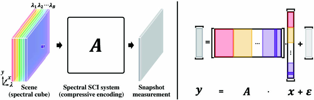
The basic idea of SCI is to encode 3D or multidimensional visual information onto 2D sensor measurement. For spectral SCI, a 3D spatio-spectral data cube is encoded to form a snapshot 2D measurement on the charge coupled device (CCD) or complementary metal oxide semiconductor (CMOS) sensor, as shown in Fig. 1.

The forward model of SCI is linear. For spectral SCI, the spectral data cube of the scene $\mathit{X}\in {\mathbb{R}}^{W\times H\times B}$, where $W$, $H$, and $B$ denote the width, height, and the number of spectral bands, respectively, is encoded onto a single 2D measurement $\mathit{Y}\in {\mathbb{R}}^{W\times H}$ (or similar size) via spectrally variant coding. By vectorizing the scene’s spectral cube and measurement, that is, $\mathit{x}=\mathrm{v}\mathrm{e}\mathrm{c}(\mathit{X})\in {\mathbb{R}}^{WHB}$ and $\mathit{y}=\mathrm{v}\mathrm{e}\mathrm{c}(\mathit{Y})\in {\mathbb{R}}^{WH}$, we can form a linear system for spectral SCI, $$\mathit{y}=\mathit{A}\mathit{x}+\mathit{\epsilon },$$(1)where $\mathit{A}\in {\mathbb{R}}^{WH\times WHB}$ and $\mathit{\epsilon }\in {\mathbb{R}}^{\mathit{WH}}$ denote the sensing matrix and the measurement/sensor noise, respectively, as shown in Fig. 1.

The spatio-spectral coding mechanism is characterized by the sensing matrix (or transport matrix from the light transport perspective), i.e., $\mathit{A}$ of the optical system, where each column of the sensing matrix $\mathit{A}$ is the vectorized image on the measurement plane by turning on the corresponding one voxel of the scene, as shown in the highlighted purple column of Fig. 1.

To encode spectral information onto a single-shot measurement, the sensing matrix must be spectrally variant. To this end, spectral SCI systems need to involve spectral dispersion devices (dispersers), like prisms, diffraction gratings, or diffusers.

Different spectral SCI systems distinguish each other by varying the coding mechanisms, which contribute to different structures of the sensing matrices. According to the coding mechanisms, i.e., the relative position of the coded mask, spectral SCI systems could be categorized into two types, i.e., image-plane coded masks and aperture-plane coded masks. The key difference here is whether one spatio-spectral voxel (e.g.,  the purple voxel on the left of Fig. 1) contributes to only one element of the sensing matrix $\mathit{A}$ or not.

For image-plane coding, the coded mask is typically located at the conjugate image plane of the sensor plane, where one spatio-spectral voxel is directly modulated by one pixel on the coded mask and then relayed to one pixel on the detector. Therefore, there is a voxel-to-pixel mapping between the scene and the corresponding column of the sensing matrix.

As mentioned before, CASSI [12,19,47,48] was the first spectral SCI system, to the best of our knowledge. And CASSI systems can be categorized into image-plane coded masks, whether they use dual dispersers or a single disperser. The key success of CASSI is to use a coded mask for spatial coding and implement a spectral shearing with a disperser (a prism [12,19,27,47,48], a grating [20], or other spectrally variant devices like spatial light modulators (SLMs) [25,49,50]) to encode 3D spatio-spectral information onto a snapshot measurement on a 2D detector.

DD-CASSI [12] preshears the spectral cube of the scene via the first prism and then spatially encodes it using a coded mask at the image plane, where the coded spectral cube is finally unsheared to match the size of the original spectral cube via the second prism. Thereby, each voxel of the scene spectral cube would correspond to one element in the sensing matrix, and the encoded spectral cube is unsheared and thus has the same spatial size as the 2D measurement thanks to the usage of two complementary prisms, as shown in the first row of Fig. 2. Single disperser, or SD-CASSI [19,47] does not preshear the scene spectral cube and only performs the spatial coding and spectral shearing with a coded mask and a prism successively, as shown in the upper part of Fig. 3. In this way, the encoded spectral cube is sheared and contains some zero rows along the shearing boundaries, as shown in the second row of Fig. 2.

The common advantage of spectral SCI systems based on an image-plane coded mask is that since one spatio-spectral voxel contributes to only one element of the sensing matrix, the final sensing matrix is a concatenation of diagonal matrices, that is, $$\mathit{A}=[{\mathit{D}}_1,\dots ,{\mathit{D}}_B],$$(2)where ${\mathit{D}}_b=\mathrm{diag}[\mathrm{vec}(C_b)]\in {\mathbb{R}}^{WH\times WH}$ with $C_b$ being the (calibrated) coded mask for the $b$th spectral band, $b=1,\dots ,B$. Therefore, $\mathit{A}{\mathit{A}}^{\top }$ is a diagonal matrix with each element the element-wise square sum of the spectrally variant coded masks, i.e., $\mathit{A}{\mathit{A}}^{\top }={\sum }_{b=1}^B{\mathit{D}}_b{\mathit{D}}_b^{\top }$. This key property of image-plane coding-based SCI systems benefits the reconstruction algorithms significantly by reducing the computational complexity, especially for projection-based algorithms [16,51]. We will focus on the SD-CASSI case for simulations and real experiments due to the efficient hardware design.

Spectral SCI systems using an aperture-plane coded mask achieve spatial encoding at the aperture plane. Each spatio-spectral voxel in the scene spectral cube is propagated to the whole sensor plane, whereas only one point is propagated for the image-plane coded mask. In this way, the sensing matrix of aperture-plane coding is a dense matrix and $\mathit{A}{\mathit{A}}^{\top }$ is generally not diagonal, thus less computationally efficient for projection-based algorithms. As a general method for spectral SCI, the proposed deep PnP prior can be integrated to tackle challenges brought by various coding mechanisms (thus being flexible) by retaining efficiency at the same time; this will be discussed in Section 3.

There are two types of implementations for aperture-plane coding of a spectral SCI. The main difference is whether the point spread function (PSF) of each spatio-spectral voxel of the scene spectral cube is spatially invariant or not. Typical spatially invariant implementations are using speckles along with memory effect [52,53] and a diffractive optical element (DOE) [28] for spatially invariant PSFs, as shown in the third row of Fig. 2. Less calibration is involved for spatially invariant implementations, which would also suffer from this assumption mismatch. Spatially variant PSFs are more general, with a ghost imaging via sparsity constraints (GISC) spectral camera [26,54] and the compact prism-based spectral camera [29] as two representatives, as shown in last row of Fig. 2. We will talk about both the algorithm for aperture-coding-based spectral SCI (Section 3.A) and the experimental results on the GISC spectral camera [54] (Section 4.B.3) as well.

Recovering 3D or multidimensional information from 2D SCI measurements is an ill-posed linear inverse problem. The main take-away from the CS [9,10,55,56] community is that sub-Nyquist sampling and reliable recovery could be achieved by constraints of the sampling/sensing matrix [55,57] and proper priors of the signal. The performance bound of the SCI-induced sensing matrix has been proved in Ref. [58]. And the fact ion that denoisers using deep neural networks could serve as the prior of natural images with certain constraints on the network training process is getting wide attention [43].

For the sparsity prior of the signal, ${\ell }_1$ norm would be sufficient for near-optimal recovery [55,56]. For natural images, or specifically spectral images, the prior distribution of natural spectral images is needed for a good recovery. From the statistical inference perspective, we can use the maximum a posteriori probability (MAP) estimate, given the measurement $\mathit{y}$ and the forward model (likelihood function $p_{y|x}$) to estimate the unknown signal $\mathit{x}$ in Eq. (1), that is, $$\begin{gathered} \widehat{\mathit{x}}=\arg {\max }_{\mathit{x}}{p}_{x|y}(\mathit{x}|\mathit{y}) \\ =\arg {\max }_{\mathit{x}}\frac{p_{y|x}(\mathit{y}|\mathit{x})p_x(\mathit{x})}{p_y(\mathit{y})} \\ =\arg {\max }_{\mathit{x}}{p}_{y|x}(\mathit{y}|\mathit{x})p_x(\mathit{x}). \end{gathered}$$(3)Given the assumption of additive white Gaussian noise (AWGN) of the measurements $\mathit{\epsilon }\sim \mathcal{N}(0,{\sigma }_{\mathit{\epsilon }}^2)$, the MAP form Eq. (3) can be rewritten as $$\begin{gathered} \widehat{\mathit{x}}=\arg {\max }_{\mathit{x}}\exp [-\frac{1}{2{\sigma }_{\mathit{\epsilon }}^2}{\Vert \mathit{y}-\mathit{A}\mathit{x}\Vert }_2^2+\log p_x(\mathit{x})] \\ =\arg {\text{min}}_{\mathit{x}}\frac{1}{2}{\Vert \mathit{y}-\mathit{A}\mathit{x}\Vert }_2^2-{\sigma }_{\mathit{\epsilon }}^2\log p_x(\mathit{x}). \end{gathered}$$(4)By replacing the unknown noise variance ${\sigma }_{\mathit{\epsilon }}^2$ with a noise-balancing factor $\lambda$ and negative log prior function $p_x(\mathit{x})$ with a regularization term $R(\mathit{x})$, Eq. (4) can be written as $$\widehat{\mathit{x}}=\arg {\text{min}}_{\mathit{x}}\frac{1}{2}{\Vert \mathit{y}-\mathit{A}\mathit{x}\Vert }_2^2+\lambda \mathit{R}(\mathit{x}).$$(5)

We further use the PnP method [40,41] based on the alternating direction method of multipliers (ADMM) [59] for image-plane coding and the two-step iterative shrinkage/thresholding (TwIST) [15] algorithm for aperture-plane coding to solve Eq. (5).

The basic idea of PnP method for inverse problems is to use a pretrained denoiser for the desired signal as a prior. It builds on the optimization-based recovery method, where the whole inverse problem is broken into easier subproblems by handling the forward-model (data-fidelity) term and the prior term separately [59] and alternating the solutions to subproblems in an iterative manner. This is why it is called the PnP method, since the denoiser could serve as a simple plug-in for the reconstruction process. Here, for spectral SCI, we use a pretrained HSI denoising network as the deep spectral prior and integrate it into an iterative optimization framework for reconstruction, as shown in the lower part of Fig. 3. We will start with the PnP–ADMM method for spectral SCI with image-plane coding, and then substitute the ADMM projection with TwIST for aperture-plane coding. Note that the difference lies in the “Projection” step in Fig. 3.

The proposed PnP method has guaranteed convergence for SCI with a bounded denoiser [42,43] and the assumption of estimated noise levels in a nonincreasing order [18].

The ADMM solution to the optimization problem Eq. (5) can be written as $${\mathit{x}}^{k+1}=\arg {\text{min}}_{\mathit{x}}\frac{1}{2}{\Vert \mathit{A}\mathit{x}-\mathit{y}\Vert }_2^2+\frac{\rho }{2}{\Vert \mathit{x}-({\mathit{z}}^k-{\mathit{u}}^k)\Vert }_2^2,$$(6)$${\mathit{z}}^{k+1}=\arg {\text{min}}_{\mathit{z}}\lambda \mathit{R}(\mathit{z})+\frac{\rho }{2}{\Vert \mathit{z}-({\mathit{x}}^{k+1}+{\mathit{u}}^k)\Vert }_2^2,$$(7)$${\mathit{u}}^{k+1}={\mathit{u}}^k+({\mathit{x}}^{k+1}-{\mathit{z}}^{k+1}),$$(8)where $\mathit{z}$ is an auxiliary variable, $\mathit{u}$ is the multiplier, $\rho$ is a penalty factor, and $k$ is the index of iterations. Recalling the proximal operator [60], defined as ${\mathrm{prox}}_g(\mathit{v})=\arg {\text{min}}_{x}g(\mathit{x})+\frac{1}{2}{\Vert \mathit{x}-\mathit{v}\Vert }_2^2$, the ADMM solution to SCI problem can be rewritten as $${\mathit{x}}^{k+1}={\mathrm{\text{prox}}}_{f/\rho }({\mathit{z}}^k-{\mathit{u}}^k),$$(9)$${\mathit{z}}^{k+1}={\mathrm{\text{prox}}}_{\lambda R/\rho }({\mathit{x}}^{k+1}+{\mathit{u}}^k),$$(10)$${\mathit{u}}^{k+1}={\mathit{u}}^k+({\mathit{x}}^{k+1}-{\mathit{z}}^{k+1}),$$(11)where $f(\mathit{x})=\frac{1}{2}{\Vert \mathit{A}\mathit{x}-\mathit{y}\Vert }_2^2$. Equation (9) is the Eulidean projection with a closed-form solution, i.e., ${\mathit{x}}^{k+1}=({\mathit{A}}^{\top }\mathit{A}+\rho \mathit{I}{)}^{-1}·[{\mathit{A}}^{\top }\mathit{y}+\rho ({\mathit{z}}^k-{\mathit{u}}^k)]$. Let ${\sigma }^2=\lambda /\rho$, and Eq. (10) can be viewed as a denoiser ${\mathcal{D}}_{\sigma }(·)$ with $\sigma$ as the estimated noise standard deviation.

Furthermore, recalling that $\mathit{A}{\mathit{A}}^{\top }$ is a diagonal matrix for image-plane coding, ${({\mathit{A}}^{\top }\mathit{A}+\rho \mathit{I})}^{-1}$ can be calculated efficiently using the matrix inversion lemma (Woodbury matrix identity) [61], i.e., $${({\mathit{A}}^{\top }\mathit{A}+\rho \mathit{I})}^{-1}={\rho }^{-1}\mathit{I}-{\rho }^{-1}{\mathit{A}}^{\top }{(\mathit{I}+\rho \mathit{A}{\mathit{A}}^{\top })}^{-1}\mathit{A}{\rho }^{-1}.$$(12)Then the Euclidean projection can be simplified and the final PnP–ADMM solution to the SCI problem [16,18,51] is $${\mathit{x}}^{k+1}=({\mathit{z}}^k-{\mathit{u}}^k)+{\mathit{A}}^{\top }[\mathit{y}-\mathit{A}({\mathit{z}}^k-{\mathit{u}}^k)]\oslash [\mathrm{D}\mathrm{i}\mathrm{a}\mathrm{g}(\mathit{A}{\mathit{A}}^{\top })+\rho ],$$(13)$${\mathit{z}}^{k+1}={\mathcal{D}}_{{\widehat{\sigma }}_k}({\mathit{x}}^{k+1}+{\mathit{u}}^k),$$(14)$${\mathit{u}}^{k+1}={\mathit{u}}^k+({\mathit{x}}^{k+1}-{\mathit{z}}^{k+1}),$$(15)where Diag(·) extracts the diagonal elements of the ensued matrix, $\oslash$ denotes the element-wise division or Hadamard division, and ${\widehat{\sigma }}_k$ is the estimated noise standard deviation for the current ($k$th) iteration. Here, the noise penalty factor $\rho$ is tuned to match the measurement (Gaussian) noise. For noiseless simulation, $\rho$ is set to 0 or a small floating-point number. For the estimated noise standard deviation for each iteration ${\widehat{\sigma }}_k$, we empirically use a large ${\widehat{\sigma }}_k$, e.g.,  50 out of 255 for the first several iterations (10 or 20 depending on the denoiser) and progressively shrink it during the iteration process, following Ref. [16].

For spectral SCI, we use a deep spectral denoiser as the prior, as detailed in Section 3.B. This is very straightforward for DD-CASSI. However, for SD-CASSI, there are spatial shifts between adjacent spectral bands because the spectrum is not unsheared by another disperser. Pratically, we calibrate spatial shifts of all spectral bands or keep the same spatial shifts for all adjacent bands and calibrate the corresponding wavelengths. We take the spatial shifts into account by unshifting the spectral bands before applying denoising and then reshifting them back to match the forward model.

As discussed in Section 2.B and Fig. 2, the sensing matrix of aperture-plane coding is dense and does not get $\mathit{A}{\mathit{A}}^{\top }$ a diagonal matrix. In this way, the matrix inversion lemma Eq. (12) will not help to simplify the calculation of the inverse ${({\mathit{A}}^{\top }\mathit{A}+\rho \mathit{I})}^{-1}$ used in ADMM. And because of the structure of aperture-plane coding, ${\mathit{A}}^{\top }\mathit{A}$ is not well-conditioned, which makes ADMM both computationally inefficient and unstable for reconstruction.

In response to the efficiency and computation stability issues caused by ADMM projection, we use one variant of the iterative shrinkage/thresholding algorithms (ISTAs) [62], i.e., TwIST [15] for aperture-plane coding. ISTA and its variants use ${\mathit{A}}^{\top }$ instead of ${\mathit{A}}^{\top }{(\mathit{A}{\mathit{A}}^{\top })}^{-1}$ for projection to avoid the matrix inversion of a large matrix $\mathit{A}{\mathit{A}}^{\top }$. In addition, TwIST employs another correction/acceleration step according to the conditioning of ${\mathit{A}}^{\top }\mathit{A}$, where the parameter could be tuned to match the measurement noise in real experiments. The final PnP–TwIST solution to the SCI problem is $${\mathit{x}}^{k+1}={\mathit{z}}^k+{\mathit{A}}^{\top }(\mathit{y}-\mathit{A}{\mathit{z}}^k),$$(16)$${\mathit{\theta }}^{k+1}={\mathcal{D}}_{{\widehat{\sigma }}_k}({\mathit{x}}^{k+1}),$$(17)$${\mathit{z}}^{k+1}=(1-\alpha ){\mathit{z}}^{k-1}+(\alpha -\beta ){\mathit{z}}^k+\beta {\mathit{\theta }}^{k+1},$$(18)where $\alpha$ and $\beta$ are the correction parameters depending on the eigenvalues of ${\mathit{A}}^{\top }\mathit{A}$, that is, $\alpha ={\widehat{\gamma }}^2+1,\beta =2\alpha /({\xi }_1+{\overline{\xi }}_m)$, whereas $\widehat{\gamma }=\frac{1-\sqrt{\kappa }}{1+\sqrt{\kappa }},\kappa ={\xi }_1/{\overline{\xi }}_m,0<{\xi }_1\le {\lambda }_i({\mathit{A}}^{\top }\mathit{A})\le {\xi }_m,{\overline{\xi }}_m=\max \{1,{\xi }_m\}$. In the experiment of GISC (Section 4.B.3), we use this PnP–TwIST due to the large scale of $\mathit{A}$. After normalization of each column, we use the default setting in the TwIST code for the related parameters.

From the idea of the PnP method for linear inverse problems, we can see that a proper denoiser could serve as a prior of optimization-based approaches, where a better denoiser would contribute to higher reconstruction quality. Deep-learning-based denoisers, especially those based on CNNs for images/videos are among the state of the art. A key challenge for using deep denoisers as priors is the flexibility in terms of data size and the input noise levels. According to Eq. (14) in PnP–ADMM and Eq. (17) in PnP–TwIST, the denoiser should be adapted to different input noise levels. Inspired by the recent advance of the fast and flexible denoising CNN (FFDNet) [46] and its success applied to video SCI [18], we propose using a deep spectral denoising network as the spatio-spectral prior, that is, the deep spectral denoising prior. The network structure of the deep spectral denoising prior is shown in Fig. 4.

The spectral image denoising problem can be formulated as $${\mathit{D}}_{\mathit{\sigma }}(\mathit{v})={\mathrm{prox}}_{{\mathit{\sigma }}^2\mathit{R}}(\mathit{v})=\arg {\text{min}}_{\mathit{x}}\mathit{R}(\mathit{x})+\frac{1}{2{\sigma }^2}{\Vert \mathit{x}-\mathit{v}\Vert }_2^2,$$(19)which basically learns the maximum prior probability of the HSIs, given the noisy image $\mathit{v}$ and the standard deviation of the Gaussian noise $\sigma$. Similar to the fast and flexible deep image denoiser [46,63] and the deep video denoiser [64], we perform spectral image denoising in a frame-wise manner following Ref. [65].

In order to consider the spectral correlation among adjacent bands, when denoising a center spectral frame with the size of $W\times H$, we take adjacent $K$ spectral frames ($K=6$ in our network) as input and stack the downsampled subimages [46,63] of all $K+1$ frames with a noise-level map initialized as the input noise standard deviation $\sigma$ to form a data cube of $\frac{W}{2}\times \frac{H}{2}\times (4K+5)$, as shown in Fig. 4. The data cube is then transported into a CNN with 14 layers ($D=14$) of convolutional layers (Conv) and the rectified linear unit (ReLU) as the activation function (except for the last layer, where nonlinearity is not needed). We use the same size of the convolutional kernel, i.e., $3\times 3$, and zero padding to retain the image size after convolution. The number of channels for the first 13 convolutional layers is set to 128 and the last one to 4, so that the output of the CNN has a size of $\frac{W}{2}\times \frac{H}{2}\times 4$. This output is rearranged to arrive a single output spectral band with its original image size $W\times H$. Hereby, we get the denoised single-band image. After looping through all spectral bands, we can get all the spectral bands denoised. To handle the boundary case of adjacent spectral frames for the first and last few bands, we use mirror padding. Note that the key to the flexibility of our algorithm is that we need to enumerate sufficient noise levels and spectral bands during training.

Our denoising network is trained on the CAVE data set [66]. It contains 32 scenes with a pixel resolution of $512\times 512$ and 31 wavelength bands from 400 to 700 nm with a step of 10 nm. We cropped patches of size $256\times 256\times 7$ from the original HSIs and employed data augmentation (rotations of 90°, 180°, 270°; vertical flip; and combinations of the above rotation and flip operations) on the extracted patches. The total number of the patches that we finally used was 30,320. We chose seven bands during training to make sure that our denoising network could take into account the high spectral correlation between adjacent bands. We use PyTorch [67] for implementation and Adam [68] as the optimizer. The total number of training epochs is set to 500, and the batch size is set to 64 with a learning rate of ${10}^{-3}$, which decays 10 times every 100 training epochs.

Regarding the noise level $\sigma$, it is set to random values between 0 and 25 out of 255 during training. Training of the entire network took approximately 2 days, using a machine equipped with an Intel i5-9400F CPU, 64 GB of memory, and an Nvidia GTX 1080 Ti GPU with 11 GB RAM.

In this section, we verify the performance of the proposed PnP algorithm by extensive experiments. First, we conduct extensive simulations to compare PnP with other competitive methods. We then apply our PnP algorithm to data captured by real spectral SCI systems. Since different systems have different settings and parameters, the excellent results of our PnP verify the flexibility of the proposed algorithm. Note that, for end-to-endCNN methods such as $\lambda$-net [37], a different network needs to be trained for each system. Moreover, since training these networks usually needs a significant amount of training data; when the system captures large-scale measurements, it will need tremendous training data and a large GPU memory, which limits the scaling performance of these end-to-end CNNs. On the other hand, our PnP algorithm can easily scale to a large data set, since the denoising is performance on patches in each iteration.

Hereby, we verify the performance of PnP by simulation using different data sets of different sizes and compare it with other popular algorithms. For the simulation data, we generate measurements following the SD-CASSI framework, as shown in the second row of Fig. 2.

We employ the publicly available data sets ICVL [69] and KAIST [35] for simulation. The ICVL data are of spatial size $1392\times 1300$ with 31 spectral bands from 400 to 700 nm at a step of 10 nm. The KAIST data are of spatial size $2704\times 3376$ with 31 spectral bands from 400 to 700 nm at a step of 10 nm. We select eight scenes of each data set, shown in Fig. 5. For both data sets, we also cropped to different spatial sizes of $256\times 256$, $512\times 512$, and $1024\times 1024$ to demonstrate the scalability of the PnP algorithm.

We compare our proposed PnP algorithm with other popular methods, including TwIST [15], generalized alternating projection based total variation minimization (GAP-TV) [51], auto-encoder (AE) [35], and U-net [70]. Note that TwIST and GAP-TV are conventional optimization methods employing the TV prior. Though TwIST has been used for a long time for CASSI-related systems, GAP-TV has recently shown a faster convergence than TwIST. AE is a deep-learning-based algorithm that takes into account the two aspects of spectral accuracy and spatial resolution. U-net is the backbone of recently proposed deep learning for spectral compressive imaging systems including $\lambda$-net [37], spatial-spectral self-attention network (TSA-net) [39], and the one used in Ref. [36].

The U-net structure basically consists of two parts, the encoder part and the decoder part. Each encoder block consists of two $3\times 3$ convolutional layers and a $2\times 2$ max pooling operation. We double the feature maps during each encoder block. After four encoder blocks, we use transposed convolution operation followed by two $3\times 3$ convolutional layers as one decoder block. We have doubled the feature maps during each decoder layer, too. We perform four blocks in the decoder and get the reconstructed result after a last additional $1\times 1$ output convolutional layer. ReLU follows each convolutional layer in both encoder and decoder as the activation function, except for the output layer, which uses the sigmoid function. Skip connections are added between the encoder blocks and decoder blocks. Similar to our denoising network, we train U-net with the CAVE data set [66]. The training process took 3 days for the spatial size of $256\times 256$. Due to the long training time and GPU memory constraints, we did not train it for larger spatial sizes up to $512\times 512$ or $1024\times 1024$. This already shows that a fixed end-to-end network such as U-net is not flexible with spatial sizes and compression ratios.

Both quantitative and qualitative metrics are used for comparison. The quantitative metrics are peak signal-to-noise ratio (PSNR) and structural similarity (SSIM) [71]. For qualitative comparison, we plot spectral frames along with spectral curves and compare them with the ground truth for visual verification. Additionally, we use Pearson correlation coefficient (corr) to assess the fidelity of recovered spectra.

From the hardware side, we use a binary random mask composed of $\{\mathrm{0,1}\}$ with the same probability. The feature size of the mask is the same as the camera. The measurement is generated following the optical path of the SD-CASSI.

For the proposed PnP algorithm, it usually needs a warm starting point to speed up the convergence. To address this, for the proposed PnP algorithm, we first run 80 iterations of GAP-TV. Since the only difference is the denoising algorithm, TV, or deep denoising, in each iteration, we only need to switch the denoising method in the flow chart, shown in Fig. 3.

The other important parameter of PnP is the noise level in each iteration. One method is to estimate the noise level in each iteration. However, this will make it computationally extensive. Therefore, similar to other PnP methods [18], we set the noise level manually in each iteration. This is also the reason we train the HSI denoising network to a wide noise range. Specifically, we set the noise level in a decreasing manner. For instance, assuming that the range of each pixel is [0,255], we set the noise level to 25 for 20 iterations, followed by 15 for 20 iterations and then tune the noise level to be smaller during the last few iterations.

Table 1 summarizes the average results of the 16 scenes shown in Fig. 5 with different spatial sizes. It can be seen that in all these three spatial sizes, PnP always leads to the best results. In particular, PnP outperforms GAP-TV by at least 2 dB in PSNR, which is the best among other algorithms. What else stands out in the table is that AE does not perform as well as in the DD-CASSI system shown in Ref. [35]. We also tested all the above algorithms using DD-CASSI; AE can achieve better results than other algorithms except PnP.Table 1.

Average PSNR (in dB), SSIM, and Running Time (in Seconds) of 16 Simulation Scenes (8 from ICVL and 8 from KAIST) at Different Spatial Sizes Using Various Algorithms^a

Regarding the running time, it can be seen that for the size of $256\times 256$, most methods only need about 2 min to reconstruct the spectral cube from a single measurement. At this small size, it is feasible to train a U-net for the end-to-end reconstruction. After training, the testing only needs 0.8 s, which is efficient in real applications. When the size gets larger, due to the limitation of GPU memory, we cannot train an end-to-end U-net, and thus we only show the results of the other four algorithms. It takes about 5–20 min to reconstruct a spectral cube with spatial size of $512\times 512$ and about 0.5 to 1 h for the size of $1024\times 1024$. In summary, PnP achieves the state-of-the-art results in a relatively short time.

Figure 6 shows the results of 31 bands of each algorithm with the spatial size of $256\times 256$ for the scene of color-checker from KAIST data set. It can be seen clearly that PnP provides the best results. Specifically, the reconstructed frames of TwIST and GAP-TV have blocky artifacts, while the frames of AE and U-net are not clean. By contrast, the frames of PnP have fine details and sharp edges. We also plot the spectral curves of several selected regions and calculate the correlations between the reconstructed spectra and the ground truth. PnP can also provide more accurate spectra. Figure 7 plots five selected spectral frames of four other scenes. Again, it is clear that PnP provides the best results.

For other sizes of the spectral cube, in order to visualize the recovered color, we convert the spectral images to synthetic-RGB (sRGB) via the International Commission on Illumination (CIE) color-matching function [72]. The results are shown in Figs. 8 and 9, respectively, for the size of $512\times 512$ and $1024\times 1024$. It can be observed that PnP outperforms other algorithms in both spatial details and spectral accuracy. Clear details and sharp edges can be recovered. Please refer to the zoomed regions of each scene.

In this section, we apply our proposed PnP algorithm into five real spectral SCI systems, namely, three SD-CASSI systems [39,47,48], one snapshot multispectral endomicroscopy [36], and a ghost spectral compressive imaging system [54]. Note that our PnP framework is using the pretrained HSI denoising network on the simulation data. Though these systems have different spatial and spectral resolutions, PnP can be used directly to all these systems. Due to the speed consideration, we only compare with TwIST and/or GAP-TV in these real data sets.

We now show three results of SD-CASSI. These measurements are captured by different systems built at different labs.•Object data consists of 33 spectral bands, each with a size of $256\times 210$ pixels. The data are captured by a CASSI system built at Duke [48]. In Fig. 10, we compare the results of PnP with TwIST. We can see that fine details can be reconstructed by PnP.•Bird data consist of 24 spectral bands, each with a size of $1021\times 703$ pixels, which are captured by another CASSI system built at Duke [47] along with the ground truth captured by a spectrometer. Figure 11 compares the reconstructed results of TwIST, GAP-TV, and PnP with the ground truth. We follow the similar procedure of shifting the reconstructed spectra two bands to keep align with optical calibration, as used in Ref. [16]. For this scene, all algorithms can provide good results, but PnP achieves the clearest frames.•Lego and Plant data consist of 28 spectral bands of size $660\times 550$, which are captured by a recently built CASSI system at Bell Labs [39]. Figures 12 and 13 show the reconstructed results of PnP, TwIST, and GAP-TV. Clearly, PnP can provide finer details than other algorithms.

Next, we apply our PnP algorithm to the snapshot multispectral endomicroscopy system built recently [36], which is a spectral SCI system plus a fiber bundle for endoscopy. It has 24 bands in the visible bandwidth, with a spatial size of $660\times 660$. We compare the results of three samples using TwIST, GAP-TV, and PnP in Fig. 14. It can be seen that both TwIST and GAP-TV lead to some noisy results, while PnP can provide clean frames.

Different from CASSI architecture, ghost imaging provides another solution to capture the spectral cube in a snapshot manner via aperture-plane coding. Hereby, we apply the PnP algorithm to the ghost imaging data captured by the system built in Ref. [54]. Since the sensing matrix of these data is large, as shown in Fig. 2, we only use the bandwidth between 510 and 660 nm with an interval of 10 nm. The spatial-spectral size of these data is $330\times 330\times 16$. The results of TwIST and PnP are shown in Fig. 15. It can be seen that PnP provides better results than TwIST, especially on the clean background.

We have developed a deep PnP algorithm for the reconstruction of spectral SCI. We trained a deep denoiser for hyper/multispectral images and plugged it to the ADMM and TwIST frameworks for different spectral CS systems. Importantly, a single pretrained denoiser can be applied to different systems with different settings. Therefore, our proposed algorithm is highly flexible and is ready to be used in different real applications. Extensive results on both simulation and real data captured by diverse systems have verified the performance of our proposed algorithm.

The running time scales linearly to the number of spectral bands because each spectral band is denoised individually by taking its neighboring $K$ bands as input to the network. There are two limitations of the proposed PnP method for spectral SCI. First, it suffers from generalization issues and data set bias, as is common for supervised approaches (for example, when applying it for remote-sensing applications with hundreds of bands, fine-tuning, or retraining on the fine spectral resolution data set). Second, sometimes it needs a good initialization to start with. Since the denoiser is trained on Gaussian noise, it might have a hard time dealing with large spatial shifts in SD-CASSI. A good initialization like GAP-TV could come to the rescue. Denoisers taking the model-induced noise into account would be desirable for this PnP method.

References

[1] B. E. Bayer. Color imaging array. U.S. patent(1976).
[18] X. Yuan, Y. Liu, J. Suo, Q. Dai. Plug-and-play algorithms for large-scale snapshot compressive imaging. Proceedings of the IEEE/CVF Conference on Computer Vision and Pattern Recognition (CVPR), 1447-1457(2020).
[37] X. Miao, X. Yuan, Y. Pu, V. Athitsos. λ-net: reconstruct hyperspectral images from a snapshot measurement. IEEE/CVF Conference on Computer Vision (ICCV), 4058-4068(2019).
[38] L. Wang, C. Sun, Y. Fu, M. H. Kim, H. Huang. Hyperspectral image reconstruction using a deep spatial-spectral prior. IEEE/CVF Conference on Computer Vision and Pattern Recognition (CVPR), 8024-8033(2019).
[39] Z. Meng, J. Ma, X. Yuan. End-to-end low cost compressive spectral imaging with spatial-spectral self-attention. European Conference on Computer Vision (ECCV), 187-204(2020).
[40] S. V. Venkatakrishnan, C. A. Bouman, B. Wohlberg. Plug-and-play priors for model based reconstruction. IEEE Global Conference on Signal and Information Processing, 945-948(2013).
[49] R. Zhu, T. Tsai, D. J. Brady. Coded aperture snapshot spectral imager based on liquid crystal spatial light modulator. Frontiers in Optics, FW1D-4(2013).
[51] X. Yuan. Generalized alternating projection based total variation minimization for compressive sensing. IEEE International Conference on Image Processing (ICIP), 2539-2543(2016).
[64] M. Tassano, J. Delon, T. Veit. FastDVDnet: towards real-time deep video denoising without flow estimation. IEEE/CVF Conference on Computer Vision and Pattern Recognition (CVPR), 1354-1363(2020).
[67] A. Paszke, H. Wallach, S. Gross, H. Larochelle, A. Beygelzimer, F. Massa, F. d’ Alché-Buc, A. Lerer, J. Bradbury, E. Fox, G. Chanan, R. Garnett, T. Killeen, Z. Lin, N. Gimelshein, L. Antiga, A. Desmaison, A. Kopf, E. Yang, Z. DeVito, M. Raison, A. Tejani, S. Chilamkurthy, B. Steiner, L. Fang, J. Bai, S. Chintala. PyTorch: an imperative style, high-performance deep learning library. Advances in Neural Information Processing Systems 32, 8024-8035(2019).
[68] D. P. Kingma, J. Ba. Adam: a method for stochastic optimization(2014).
[69] B. Arad, O. Ben-Shahar. Sparse recovery of hyperspectral signal from natural RGB images. European Conference on Computer Vision, 19-34(2016).
[70] O. Ronneberger, P. Fischer, T. Brox. U-net: convolutional networks for biomedical image segmentation. International Conference on Medical Image Computing and Computer-Assisted Intervention, 234-241(2015).