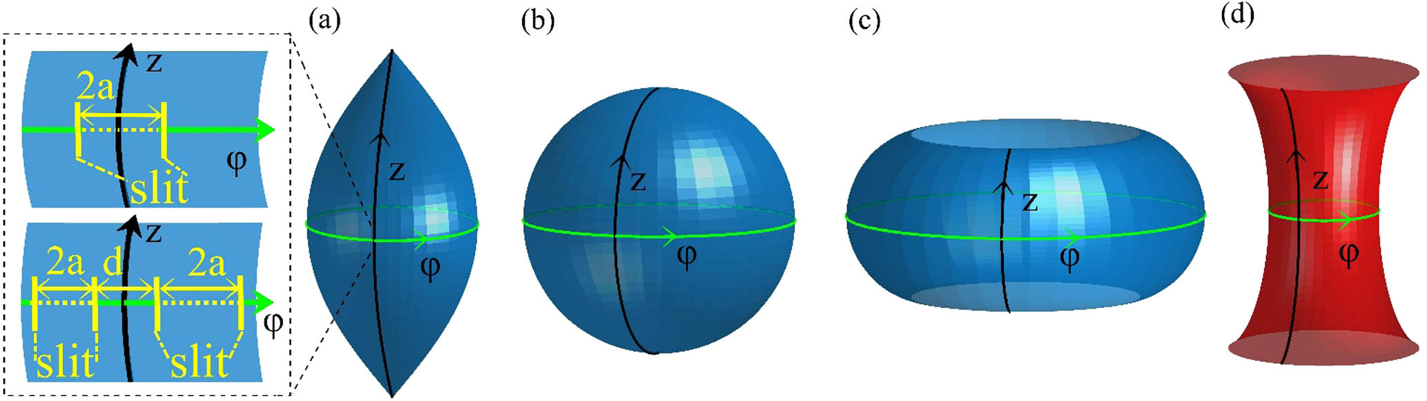
Fig. 1. SORs with constant (a)–(c) positive and (d) negative Gaussian curvature K. Here (a) spindle with r0<R, (b) sphere with r0=R, and (c) bulge with r0>R, where R=|K|−12 is the radius of Gaussian curvature, and r0 is an initial rotational radius (or radius of equator) at z=0. The black/green solid lines are the lines of longitude/equator. The inset on the left side of (a) shows the schematic of a single slit (up) and double slits (down) on surface, which are located at the equator (z=0).

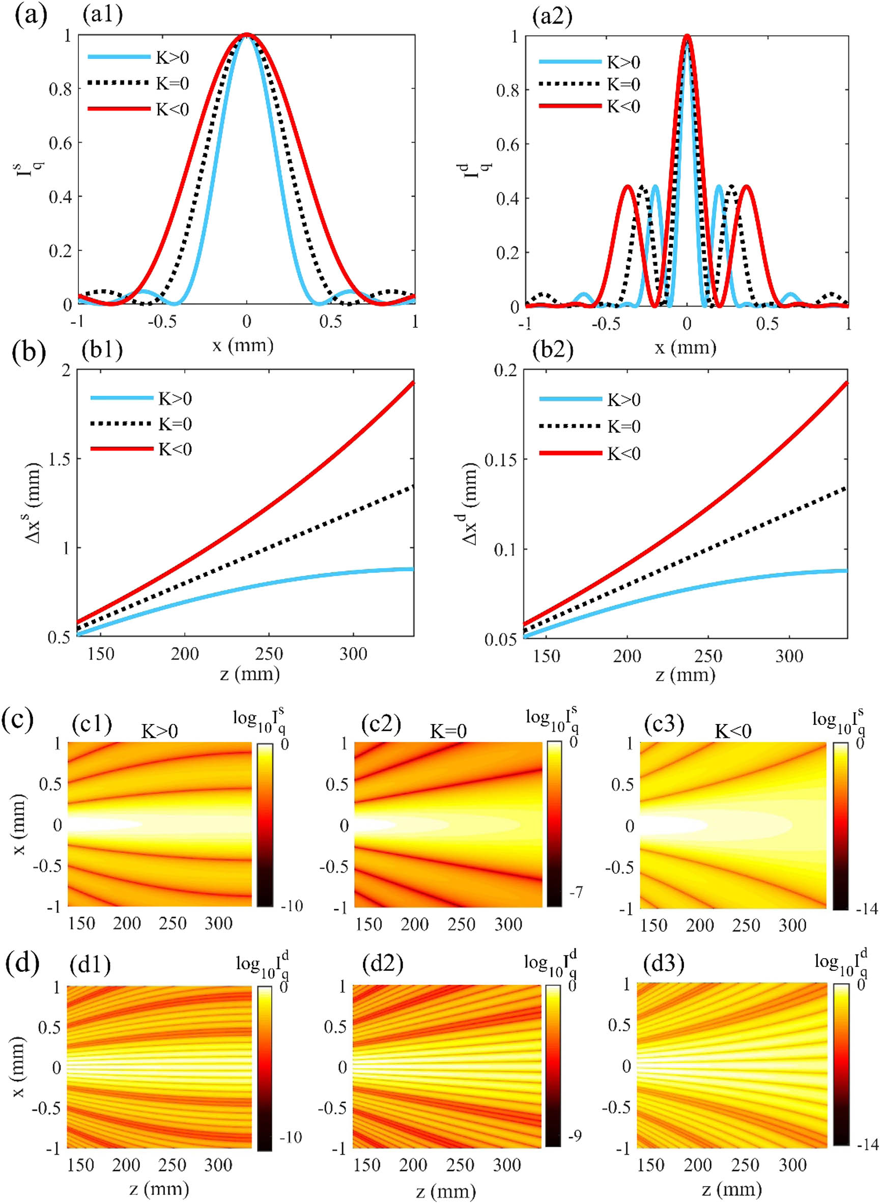
Fig. 2. Diffraction and interference on curved space. (a) Intensity distributions of Fraunhofer (a1) single-slit diffraction and (a2) double-slit interference of light at z=300  mm on SORs with different Gaussian curvature. (b) Variations of the central fringe widths Δxs and Δxd for (b1) single-slit diffraction and (b2) double-slit interference with the propagation distance in different SORs. (c), (d) Evolutions of light fields of Fraunhofer (c) single-slit diffraction and (d) double-slit interference in different spaces: (c1), (d1) K>0, (c2), (d2) K=0, and (c3), (d3) K<0. Here the parameters for SORs with R=220  mm are taken as K=20.66  m−2 for K>0, and K=−20.66  m−2 for K<0. Other parameters are λ=400  nm, r0=100  mm, a=0.1  mm, d=0.2  mm in (a2) and d=0.8  mm in (d1)–(d3) for better visualization.

Fig. 3. Effect of Gaussian curvature K of SORs on the change of the diffraction limit at different propagation distance z. The black dashed line denotes the case for the diffraction limit in flat space. The zero value of δ means no effect on diffraction limit, compared with the case in flat space.

Fig. 4. Diffraction of light fields along different propagation directions on (a) spindle, (b) sphere, and (c) hyperboloid. The propagation direction is described by the angle Θ between the longitude (black solid lines) and the incident direction. Here three typical propagation directions with Θ=30°, 45°, and 60° are considered, and the corresponding geodesics are indicated by the white, yellow, and green curves. D is the propagation distance along these geodesics. The initial central position of the input plane is zi=−230.384  mm, −295.134  mm, and −166.415  mm in (a)–(c), respectively, the parameters of these SORs are r0=100  mm, 220 mm, and 100 mm in (a)–(c), respectively, and other parameters are the same as in Fig. 2.

Fig. 5. Diffraction of light fields along different propagation directions on (a) an FP surface, (b) a SdS2 surface, and (c) a PPSS surface. The propagation direction Θ is defined the same as in Fig. 4, and three typical directions Θ=3°, 9°, and 15°, corresponding to the white, yellow, and green geodesics, respectively, are plotted. The surfaces are colored by blue/red to indicate the regions with positive/negative Gaussian curvature. The black dotted lines in (a3), (b3), and (c3) show the variation of diffraction limit in flat space. Here the initial central positions of the input plane are ri=460  mm in (a), ri=283.66  mm in (b), and zi=100  mm in (c), the Schwarzschild radius rs=30  mm in (a) and (b), and the cosmological constant is Λ=33.33  m−2 in (b). In (c), we take α=100  mm, B=10  mm, β=20  mm, and ε=−1.25π. Other parameters are the same as in Fig. 2.

Fig. 6. Dependence of the relative quantity δ on the propagation direction at different propagation distances (a) D=400  mm and (b) D=500  mm. Other parameters are the same as in Figs. 4 and 5.