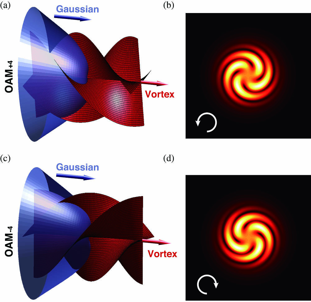
Fig. 1. (a) and (c) are the interference principles between Gaussian beams and VBs with l = +4 and l = −4, respectively. (b) and (d) are obtained interferograms corresponding to l = +4 and l = −4.

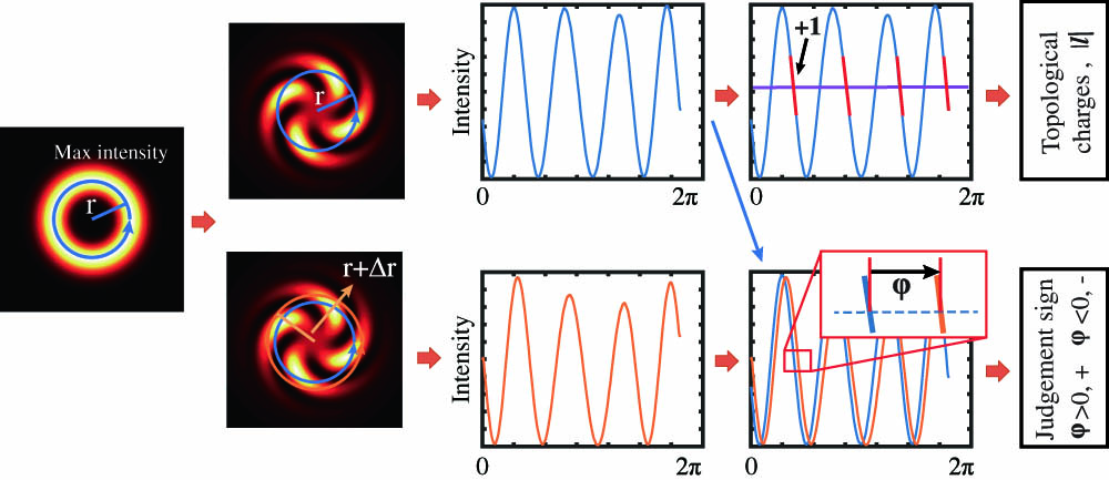
Fig. 2. Recognition principle of OAM mode: OAM mode equals the number of intersections between the average value and the falling edge of the waveform, and the mode sign is determined by comparing the phase difference of the waveform at the radii r and r + Δr.

Fig. 3. Schematic diagram of OAM-FSO communication system with VIR-GSF demodulation technique under the free-space AT channel.

Fig. 4. Filtering effect of GSF at different levels m, where m is set as 15 and 25. The comparison of waveforms after GSF operation and the original waveform is given.

Fig. 5. Intensity distribution and interferogram of the VBs when the transmission distance is 1 km, where (a), (b), and (c) represent the weak, medium, and strong-turbulence levels, respectively.

Fig. 6. Recognition accuracy of various turbulence levels when the transmission distance is 1 km. (a) shows the accuracy under no-turbulence, weak-turbulence, and medium-turbulence conditions. (b) shows that the recognition accuracy and average accuracy under the conditions of medium-strong and strong turbulence.

Fig. 7. (a) Recognition accuracy of the VIR-GSF scheme at the conditions of no turbulence, weak turbulence, and medium turbulence. The recognition accuracy and average accuracy under (b) medium-strong and (c) strong-turbulence conditions. (d) Comparison of performance of CNN, CNN-GS, and VIR-GSF schemes in a turbulent environment for transmission of 2 km.

Table 1. The Proposed VIR-GSF Algorithm