• Chinese Optics Letters
  • Vol. 20, Issue 2, 020601 (2022)
Lin Zhao1、2, Yuan Hao1, Li Chen1, Wenyi Liu1, Meng Jin1, Yi Wu1, Jiamin Tao1, Kaiqian Jie1, and Hongzhan Liu1、*
Author Affiliations
  • 1Guangdong Provincial Key Laboratory of Nanophotonic Functional Materials and Devices, Guangzhou 510006, China
  • 2School of Electronics and Information Technology, Sun Yat-sen University, Guangzhou 510275, China
  • show less
    DOI: 10.3788/COL202220.020601 Cite this Article Set citation alerts
    Lin Zhao, Yuan Hao, Li Chen, Wenyi Liu, Meng Jin, Yi Wu, Jiamin Tao, Kaiqian Jie, Hongzhan Liu. High-accuracy mode recognition method in orbital angular momentum optical communication system[J]. Chinese Optics Letters, 2022, 20(2): 020601 Copy Citation Text show less

    Abstract

    Vortex optical communication has been a hot research field in recent years. A key step is mode recognition in the orbital angular momentum (OAM) free-space optical (FSO) communication system. In this article, we propose an OAM mode recognition method based on image recognition technology, which uses the interferogram between the vortex beam and the Gaussian beam to identify the OAM mode. In order to resist the influence of atmospheric turbulence on the recognition accuracy, we added a Gaussian smoothing filter into the recognition process. Moreover, we used random phase screens to generate interferogram sets at distances of 1 km and 2 km. The verification result shows that the proposed scheme produces high identification accuracy for the distorted optical field. The average accuracy can reach 100% and 87.78% under the conditions of medium- and strong-turbulence levels, respectively. It is anticipated that these results might be helpful for improving the reliability of the OAM-FSO communication system in the future.

    1. Introduction

    Nowadays, vortex beams (VBs), carrying orbital angular momentum (OAM), have been known as the hot spots and shown great potential in various fields such as optical micro-manipulation, optical sensors, optical transmission, optical lasers, and amplifiers[1]. In 1992, Allen et al. indicated that for beams with helical phase fronts of exp(ilϕ) the OAM in the propagation direction has the discrete values of lh per photon, where h is the reduced Planck constant, and l is usually an integer that represents the topological charge (TC), whose sign indicates the direction of the phase spiral[2]. In theory, the VBs with different OAM modes are mutually orthogonal, and their intensity distribution presents unique “doughnut” shapes due to phase uncertainty at the beam cross section[3]. The discovery of optical vortices carrying OAM has accelerated progress in many research areas[4]. Especially in optical communications, VBs are of great potential in increasing capacity and modulation ability by providing additional physical dimension[5]. By multiplexing VBs, the transmission rate of Tbit/s is realized in free-space optical (FSO) communication[6,7]. Also, further studies have shown that hybrid multiplexing of OAM and other dimensions can achieve communication capacity close to Pbit/s[8]. However, the OAM shift keying communication, which encodes digital signals to OAM modes, is severely hampered because the locking effective detection methods can hardly adapt to the fast switching modes. Moreover, the VBs are susceptible to atmospheric turbulence (AT), which may cause wavefront distortion and lead to mode diffusion[9]. Hence, fast and high-accuracy OAM mode recognition is a challenge in the practical application of VBs.

    Many schemes have been proposed to detect OAM modes. The most common schemes are interference and diffraction methods[10]. Through the interference of VBs with the Gaussian beams or planar wave, the TC information can be extracted from the interference fringes. There are two main schemes for using machines to recognize interference fringes: traditional machine learning and deep learning technology[11]. Unfortunately, the effects of AT undermine the performance of simple image recognition technologies, which causes poor recognition accuracy. Meanwhile, most machine learning schemes are based on convolutional neural network (CNN)[12], which usually requires complex network architecture and huge computational cost. Therefore, the combination of reduction in computational complexity and anti-turbulence capability has become top priority.

    In this article, we proposed and designed an OAM mode recognition method based on an interferogram processed by a Gaussian smoothing filter (GSF) to identify the OAM modes of VBs. This method is called vortex interferogram recognition (VIR) based on GSF, which is abbreviated as VIR-GSF in this article. Performing simple image feature extraction on the VB light field, this scheme realizes mode recognition. Without a complex convolution and deconvolution process, the computational cost is greatly reduced. Since GSF can strengthen the stability of optical field distribution and reduce the variance of intensity fluctuations, by adding GSF to process the interferogram between the Gaussian beam and the VB, high identification accuracy for the distorted image disturbed by turbulence can be obtained. The calculation results show that this scheme has high accuracy for 1 km transmission in turbulent channels. Specifically, in no-turbulence, weak-turbulence (Cn2=1×10¹⁶m2/3), and medium-turbulence (Cn2=1×10¹⁵m2/3) conditions, the identification rate is up to 100%. Under strong-turbulence (Cn2=1×10¹⁴m2/3) conditions, the recognition accuracy can reach 91.24%. Moreover, the proposed scheme is compared with two reference schemes, i.e., the traditional CNN algorithm and the CNN with Gerchberg–Saxton (GS) algorithm[13], and our scheme can achieve better performance.

    2. Methods

    At the receiver end of the OAM communication system, various OAM modes of the VB need to be demodulated. High-accuracy recognition of OAM modes is a necessary prerequisite for accurately distinguishing different modes. In the proposed scheme, mode recognition is accomplished based on the phase information carried by the VBs[14]. Firstly, the VBs interfere with the Gaussian beam to convert the phase information into intensity distribution, and they use a photon detector to detect the intensity signals[15]. In this process, we need to collect both intensity images and interferograms. The principle of interference between the VB and Gaussian beam is shown in Fig. 1, and the expression of the interference optical field E is[16]E=ELG+ETEM00.

    (a) and (c) are the interference principles between Gaussian beams and VBs with l = +4 and l = −4, respectively. (b) and (d) are obtained interferograms corresponding to l = +4 and l = −4.

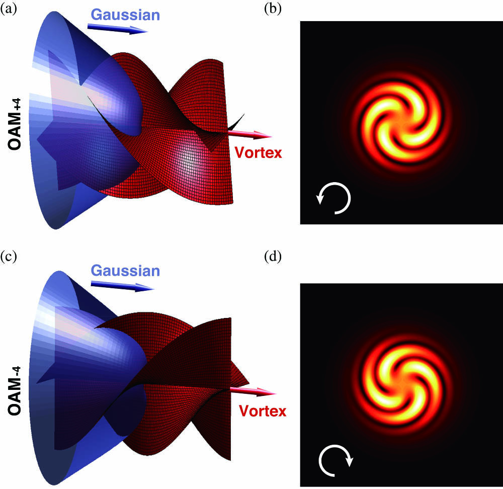
    Figure 1.(a) and (c) are the interference principles between Gaussian beams and VBs with l = +4 and l = −4, respectively. (b) and (d) are obtained interferograms corresponding to l = +4 and l = −4.

    Among them, the first item ELG is used to generate the Laguerre–Gaussian beam, which is one of the classic VBs. The cylindrically symmetric solutions ELG(r,φ,z) are given by[2,17]ELG(r,φ,z)=2p!π(p+|l|)!1ω2(z)[2rω2(z)]|l|Lp|l|[2r2ω2(z)]×exp[i(2p+|l|+1)arctan(zzR)]×exp[r2ω(z)ikr2z2R(z)]exp(ilφ).

    The second item ETEM00 is the optical field distribution of the fundamental mode Gaussian beam, and its expression is as follows: ETEM00(r,φ,z)=1ω2(z)exp[r2ω(z)ikr2z2R(z)]×exp[iarctan(zzR)].

    In the above expressions, l and p are the order of the OAM mode and radial index, respectively, the wavenumber k=2π/λ with λ as the wavelength, and Lp|l|(·) is the generalized Laguerre polynomial. ω0 is the size of the beam waist, ω(z)=ω01+(z/zR)2 is the radius of the beam, and zR=πω02/λ is the Rayleigh range. φ is the azimuth angle, and R(z) describes the curvature of the spherical wave near the optical axis.

    After the realization of Eqs. (1) and (2), the intensity images F1 and interferograms F2 of VBs are obtained. Further, we adopt an intensity map to calculate the average amplitude value of light intensity on the ring with different radii from the center outward. Then, the MAX{·} function is used to get the r value corresponding to the largest average amplitude. Each pair of interference and intensity images is from the same VB, so their intensity and phase have a one-to-one correspondence. We utilize r of the maximum amplitude in the interference image to find a circle with a radius of r and extract the intensity value on the circle corresponding to the radius r to create a one-dimensional matrix Mr. The waveform is plotted along a one-dimensional matrix, and the number of fluctuations of the waveform represents the absolute value of the OAM mode |l|. Specifically, |l| is equal to the number of intersections between the average intensity A(r) and the falling edge of the waveform Mr. The detailed recognition principle of this scheme is explained in Fig. 2. Next, we need to determine the sign of the OAM modes. We extract another one-dimensional matrix Mr+Δr from the ring with radius r+Δr in the same interferogram, where Δr needs to satisfy the following conditions: 0<Δr<2π·R(z)/(k·z).

    Recognition principle of OAM mode: OAM mode equals the number of intersections between the average value and the falling edge of the waveform, and the mode sign is determined by comparing the phase difference of the waveform at the radii r and r + Δr.

    Figure 2.Recognition principle of OAM mode: OAM mode equals the number of intersections between the average value and the falling edge of the waveform, and the mode sign is determined by comparing the phase difference of the waveform at the radii r and r + Δr.

    Equation (4) guarantees that the phase difference φ between matrices Mr and Mr+Δr satisfies π/2<φ<π/2. If φ>0, the sign of the OAM mode is positive. If φ<0, the sign is negative. Combining the above two steps, the OAM state can be determined jointly by the absolute value and the sign. However, the waveforms will be influenced by AT. So, we simulated turbulence and added this artificial turbulence into the beam propagation process. The influence of AT on the OAM beam can be approximate to the effect caused by a series of random phase screens along the propagation path. Among them, every random phase screen is a thin sheet that can change the phase distribution of the transmitted beam, and its perturbation of the refractive index is approximately represented by the Kolmogorov spectrum[18]. The power spectral models of refractive-index fluctuations in each phase screen can be expressed as ϕ(kx,ky)[17]: ϕ(kx,ky)=0.033Cn2[1+1.802kx2+ky2kl20.254(kx2+ky2kl2)7/12]×exp(kx2+ky2kl2)(kx2+ky2+1L02)11/6,where Cn2 is the structure constant of the refractive index (in units of m2/3), which is used to describe the AT intensity. kx and ky are the wavenumber in the x and y directions, respectively. The L0 and l0 are the outer scale and inner scale of AT, kl=3.3/l0. Further, the fluctuation spectrum will affect the wavefront phase of the OAM beam. The variance of the phase spectrum can be written as ψ2(kx,ky)=2πΔz·(kx2+ky2)·ϕ(kx,ky)·(2πNΔx)2,where N and Δx represent the size and grid spacing of the random phase screens, respectively. What is more, Δz is the interval distance between adjacent phase screens. To facilitate the calculation, the random distribution of phase perturbation is described in the Cartesian coordinate system, and the phase screen is then expressed in the frequency domain through the fast Fourier transform (FFT) operation. θ(x,y) is an N×N phase screen (N=500), which can be expressed as follows: θ(x,y)=F{Cψ(kx,ky)},where F{·} is FFT, C is a complex random matrix with a mean of zero and a variance of one. Through the above turbulence simulation model, the intensity maps after AT disturbance are obtained. Next, after the VB interferes with the Gaussian beam, the interferogram is eventually obtained. The principle of the VB generation and interference under turbulence is shown in Fig. 3.

    Schematic diagram of OAM-FSO communication system with VIR-GSF demodulation technique under the free-space AT channel.

    Figure 3.Schematic diagram of OAM-FSO communication system with VIR-GSF demodulation technique under the free-space AT channel.

    In order to reduce the influence of random scattering on the VBs, we added GSF in the recognition process to optimize the waveform jitter of the matrices Mr and Mr+Δr. It should be emphasized that executing GSF has great significance for extracting waveforms, which can effectively improve the recognition accuracy. The specific operation of GSF is calculating the weighted average of the pixel values within the neighborhood and then saving the value to new matrices M¯r and M¯r+Δr. The Gaussian smoothing can be described as y¯j=1ki=mmexp[(xixj)22σ2]yi,0<j<n,2m<n,with k=i=mmexp[(xixj)22σ2],where σ is the smoothing factor, and (xi,yi) are elements in matrix Mr. n is the size of matrix Mr, and m represents the smoothness level. When m increases, the GSF’s ability to filter noise will become stronger, but the loss of features that are helpful with identifying the waveform will also be more obvious. Therefore, choosing an appropriate m determines the success rate of mode recognition. In this study, we took two cases of m=15 and m=25 as examples and compared their effectiveness. The comparison results of smoothness are shown in Fig. 4. From the results, we find that the original waveform is unstable because the received beam additionally carries some random disturbance and noise. By performing GSF, sawtooth waves and noise signals are reduced. The waveform of matrix M¯r becomes smoother and more stable. However, an unlimited increase in m is disadvantageous, and a larger m will bring greater loss of effective information. So, we finally chose m=25 as the smoothness level.

    Filtering effect of GSF at different levels m, where m is set as 15 and 25. The comparison of waveforms after GSF operation and the original waveform is given.

    Figure 4.Filtering effect of GSF at different levels m, where m is set as 15 and 25. The comparison of waveforms after GSF operation and the original waveform is given.

    Combining our proposed VIR scheme and using GSF can realize OAM mode recognition under AT environment. As a brief summary, we outline the proposed VIR-GSF scheme in Algorithm 1.

    1: Input: intensity images F1(N×N) and interferograms F2(N×N)
    2: Convert F1(N×N), F2(N×N) to grayscale image as F1(N×N), F2(N×N)
    3: forR = 1:1:N/2 do
    4: Extract elements on circle with radius R from F1(N×N) as MR
    5:  A(R) = mean(MR)
    6: end for
    7: r = {R|A(R) = MAX{A}}
    8: Extract elements on circle with radius r from F2(N×N) as Mr
    9: Extract elements on circle with radius (r + Δr) from F2(N×N) as Mrr
    10: M¯r=GSF{Mr|m = 25}
    11: M¯r+Δr=GSF{Mrr|m = 25}
    12: Compare the phase difference φ between M¯r and M¯r+Δr
    13: ifφ>0then
    14:  s = +1
    15: else
    16:  s = −1
    17: end if
    18: Calculate |l| by intersections between curves M¯r and A(r)
    19: l = s × |l|
    20: Return: OAM mode l

    Table 1. The Proposed VIR-GSF Algorithm

    3. Simulations and Results

    In the numerical simulation, we used five levels of AT intensity: no turbulence, weak turbulence, medium turbulence, medium-strong turbulence (Cn2=5×10¹⁵m2/3), and strong turbulence. The transmission distance used two cases of 1 km and 2 km. Figure 5 shows the image sets at 1 km, and the number of images in each mode is 1000. These images will be used to test the accuracy of the proposed scheme.

    Intensity distribution and interferogram of the VBs when the transmission distance is 1 km, where (a), (b), and (c) represent the weak, medium, and strong-turbulence levels, respectively.

    Figure 5.Intensity distribution and interferogram of the VBs when the transmission distance is 1 km, where (a), (b), and (c) represent the weak, medium, and strong-turbulence levels, respectively.

    When the transmission distance is 1 km, the recognition accuracy of the VIR-GSF scheme is shown in Fig. 6. Under the conditions of no turbulence, since the beam is stable, and its phase distribution is uniform, the mode identification accuracy can reach 100%. When the AT intensity is increased to weak and medium levels, recognition accuracy can be maintained at 100%, and the results are shown in Fig. 6(a). Further increasing the AT intensity to medium-strong and strong levels, the average accuracy can still reach 98.02% and 91.24%, as shown in Fig. 6(b).

    Recognition accuracy of various turbulence levels when the transmission distance is 1 km. (a) shows the accuracy under no-turbulence, weak-turbulence, and medium-turbulence conditions. (b) shows that the recognition accuracy and average accuracy under the conditions of medium-strong and strong turbulence.

    Figure 6.Recognition accuracy of various turbulence levels when the transmission distance is 1 km. (a) shows the accuracy under no-turbulence, weak-turbulence, and medium-turbulence conditions. (b) shows that the recognition accuracy and average accuracy under the conditions of medium-strong and strong turbulence.

    When the transmission distance is 2 km, the test results are shown in Figs. 7(a)7(c). The results show that the accuracy can still be maintained at 100% under no-turbulence, weak-turbulence, and medium-turbulence conditions. Upgrading the turbulence level to medium-strong and strong degrees, the accuracy can reach 96.36% and 87.73%, respectively.

    (a) Recognition accuracy of the VIR-GSF scheme at the conditions of no turbulence, weak turbulence, and medium turbulence. The recognition accuracy and average accuracy under (b) medium-strong and (c) strong-turbulence conditions. (d) Comparison of performance of CNN, CNN-GS, and VIR-GSF schemes in a turbulent environment for transmission of 2 km.

    Figure 7.(a) Recognition accuracy of the VIR-GSF scheme at the conditions of no turbulence, weak turbulence, and medium turbulence. The recognition accuracy and average accuracy under (b) medium-strong and (c) strong-turbulence conditions. (d) Comparison of performance of CNN, CNN-GS, and VIR-GSF schemes in a turbulent environment for transmission of 2 km.

    In addition, the proposed VIR-GSF scheme is compared with two reference methods of CNN and CNN-GS. The traditional CNN algorithm includes the input layer (N×N), convolutional layer (CL) 1 (28×28), pooling layer (PL) 1 (max pooling, 12×12), CL 2 (8×8), PL 2 (4×4), fully connected layer (FCL) 1 (50 nodes), FCL 2 (50 nodes), and output layer. The CNN-GS scheme adds the GS algorithm basis on the traditional CNN scheme. The comparison results of average accuracy are shown in Fig. 7(d). In this case of weak turbulence, their recognition accuracy can reach 100%. When increasing turbulence intensity from the weak to the medium level, the accuracy of the CNN scheme drops to 95.6%. In a strong-turbulence environment, the recognition accuracies of CNN, CNN-GS, and VIR-GSF are 74%, 81.34%, and 87.73%. Therefore, our proposed VIR-GSF scheme has better performance than the CNN and CNN-GS schemes.

    4. Conclusion

    In this Letter, an OAM modes recognition method based on an interferogram was proposed. This method realizes the OAM modes recognition by computing the number of intersections between the average value and the falling edges of the waveform. Additionally, the GSF algorithm is adopted to reduce the influence of AT on OAM-FSO communication. The VIR-GSF scheme can achieve higher recognition accuracy in turbulent environments without using neural networks. This scheme can greatly save computational resources and reduce system complexity. It is anticipated that our work might be helpful for further improving the reliability of the OAM-FSO communication system.

    References

    [1] Y. Shen, X. Wang, Z. Xie, C. Min, Q. Liu, M. Gong, X. Yuan. Optical vortices 30 years on: OAM manipulation from topological charge to multiple singularities. Light Sci. Appl., 8, 90(2019).

    [2] L. Allen, M. W. Beijersbergen, R. Spreeuw, R. J. C. Spreeuw, J. P. Woerdman. Orbital angular momentum of light and the transformation of Laguerre–Gaussian laser modes. Phys. Rev. A, 45, 8185(1992).

    [3] L. Chen, R. K. Singh, A. Dogariu, Z. Chen, J. Pu. Estimating topological charge of propagating vortex from single-shot non-imaged speckle. Chin. Opt. Lett., 19, 022603(2021).

    [4] Y. Shen, Z. Shen, G. Zhao, W. Hu. Photopatterned liquid crystal mediated terahertz Bessel vortex beam generator. Chin. Opt. Lett., 18, 080003(2020).

    [5] A. E. Willner, H. Huang, Y. Yan, Y. Ren, N. Ahmed, G. Xie, C. Bao, L. Li, Y. Cao, Z. Zhao, J. Wang, M. Lavery, M. Tur, S. Ramachandran, A. Molisch, N. Ashrafi, S. Ashrafi. Optical communications using orbital angular momentum beams. Adv. Opt. Photon., 7, 66(2015).

    [6] J. Wang, J. Yang, I. Fazal, N. Ahmed, Y. Yan, H. Huang, Y. Ren, Y. Yue, S. Dolinar, M. Tur, A. E. Willner. Terabit free-space data transmission employing orbital angular momentum multiplexing. Nat. Photon., 6, 488(2012).

    [7] L. Zhao, T. Jiang, M. Mao, Y. Zhang, H. Liu, Z. Wei, D. Deng, A. Luo. Improve the capacity of data transmission in orbital angular momentum multiplexing by adjusting link structure. IEEE Photon. J., 12, 5501111(2020).

    [8] J. Wang, S. Li, M. Luo, J. Liu, L. Zhu, C. Li, D. Xie, Q. Yang, S. Yu, J. Sun, X. Zhang, W. Shieh, A. WillnerEuropean Conference on Optical Communication (ECOC). N-dimentional multiplexing link with 1.036-Pbit/s transmission capacity and 112.6-bit/s/Hz spectral efficiency using OFDM- 8QAM signals over 368 WDM pol-muxed 26 OAM modes(2014).

    [9] Q. Tian, L. Zhu, Y. Wang, Q. Zhang, B. Liu, X. Xin. The propagation properties of a longitudinal orbital angular momentum multiplexing system in atmospheric turbulence. IEEE Photon. J., 10, 7900416(2018).

    [10] L. Chen, W. Zhang, Q. Lu, X. Lin. Making and identifying optical superposition of very high orbital angular momenta. Phys. Rev. A, 88, 4019(2013).

    [11] D. Zibar, M. Piels, R. Jones, C. G. Schaeffer. Machine learning techniques in optical communication. J. Lightwave Technol., 34, 1442(2016).

    [12] T. Doster, A. T. Watnik. Machine learning approach to OAM beam demultiplexing via convolutional neural networks. Appl. Opt., 56, 3386(2017).

    [13] M. I. Dedo, Z. Wang, K. Guo, Z. Guo. OAM mode recognition based on joint scheme of combining the Gerchberg–Saxton (GS) algorithm and convolutional neural network (CNN). Opt. Commun., 456, 124696(2020).

    [14] P. Li, B. Wang, X. Song, X. Zhang. Non-destructive identification of twisted light. Opt. Lett., 41, 1574(2016).

    [15] S. Zhao, J. Leach, L. Gong, J. Ding, B. Zheng. Aberration corrections for free-space optical communications in atmosphere turbulence using orbital angular momentum states. Opt. Express, 20, 452(2012).

    [16] J. Vickers, M. J. Burch, R. Vyas, S. Singh. Phase and interference properties of optical vortex beams. J. Opt. Soc. Am. A, 25, 823(2008).

    [17] T. Doster, A. T. Watnik. Laguerre–Gauss and Bessel–Gauss beams propagation through turbulence: analysis of channel efficiency. Appl. Opt., 55, 10239(2016).

    [18] L. C. Andrews, R. L. Phillips. Laser Beam Propagation through Random Media(2005).

    Lin Zhao, Yuan Hao, Li Chen, Wenyi Liu, Meng Jin, Yi Wu, Jiamin Tao, Kaiqian Jie, Hongzhan Liu. High-accuracy mode recognition method in orbital angular momentum optical communication system[J]. Chinese Optics Letters, 2022, 20(2): 020601
    Download Citation