
Yan-Lei Shang, Ming-Yong Ye, Xiu-Min Lin, "Experimental observation of Fano-like resonance in a whispering-gallery-mode microresonator in aqueous environment," Photonics Res. 5, 119 (2017)
- Photonics Research
- Vol. 5, Issue 2, 119 (2017)
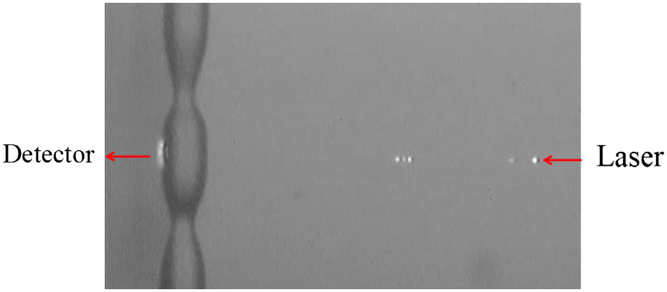
Fig. 1. Micrograph of the SLM immersed in water. The fiber taper is placed under the SLM and some scattering points on it are clearly shown.
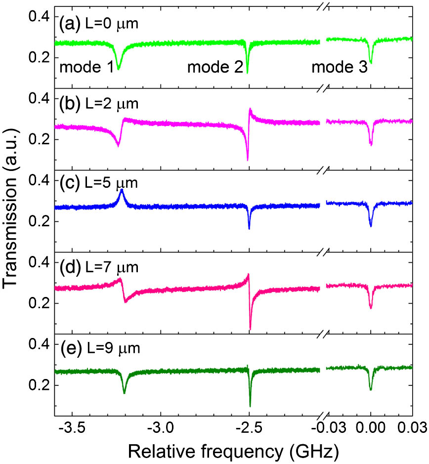
Fig. 2. Experimental transmission spectra with different positions of the SLM. From top to bottom, the SLM was moved to the left along the fiber taper.
Fig. 3. Microresonator side-coupled to a waveguide. The waveguide together with the embedded partially reflecting element simulates the function of the fiber taper in the experiment.
Fig. 4. Simulation of the dependence of the line shape of mode 1 on the position of the SLM. Increasing the value of θ k o 1 / 2 π = 2.6 MHz k e 1 / 2 π = 420.0 MHz k 1 = k o 1 + k e 1 k o 2 / 2 π = 2.5 MHz k e 2 / 2 π = 19.8 MHz g / 2 π = 19.2 MHz r = 0.42
Fig. 5. Simulation of the dependence of the line shape of mode 2 on the position of the SLM. Increasing the value of θ k o 1 / 2 π = 2.3 MHz k e 1 / 2 π = 260.0 MHz k 1 = k o 1 + k e 1 k o 2 / 2 π = 2.1 MHz k e 2 / 2 π = 4.0 MHz g / 2 π = 21.4 MHz r = 0.42
Fig. 6. Comparison between the experimental line shapes and simulated line shapes for mode 1. Experimental line shapes are normalized and shifted for clarity. Simulated line shapes are also shifted and they are plotted using the same parameters as those in Fig. 4 .
Fig. 7. Comparison between the experimental and simulated line shapes for mode 2. Experimental line shapes are normalized and shifted for clarity. Simulated line shapes are also shifted and they are plotted using the same parameters as those in Fig. 5 .


Set citation alerts for the article
Please enter your email address

© Copyright 2018-2021 | Chinese Laser Press. All Rights Reserved 沪ICP备15018463号-20