• Photonics Research
  • Vol. 11, Issue 12, 2072 (2023)
Zhiming Tian1, Ming Zhao1、*, Dong Yang2, Sen Wang1, and An Pan3、4、5
Author Affiliations
  • 1College of Information Science Technology, Dalian Maritime University, Dalian 116026, China
  • 2China Academy of Space Technology, Beijing 100086, China
  • 3State Key Laboratory of Transient Optics and Photonics, Xi’an Institute of Optics and Precision Mechanics, Chinese Academy of Sciences, Xi’an 710119, China
  • 4University of Chinese Academy of Sciences, Beijing 100049, China
  • 5e-mail: panan@opt.cn
  • show less
    DOI: 10.1364/PRJ.493938 Cite this Article Set citation alerts
    Zhiming Tian, Ming Zhao, Dong Yang, Sen Wang, An Pan. Optical remote imaging via Fourier ptychography[J]. Photonics Research, 2023, 11(12): 2072 Copy Citation Text show less
    (a) Proposed scheme. The object is illuminated by a divergent laser beam to increase the FOV. The scattering from the object is recorded by the sensor via an imaging lens. As the numerical aperture of the imaging system is fixed, a limited resolution image is obtained on the sensor plane. (b) FP raw images. By shifting the laser source with an x-y moving stage, a sequence of raw images is captured. An example of a raw image is blurred and degraded by speckles. Using the captured image sequence, the super-resolution reconstruction can be achieved with the proposed method. The FP reconstruction in (c) reduces the speckle size and improves the resolution. A speckle denoising algorithm is further performed to improve the quality of the reconstruction, and its denoising image is shown in (d).
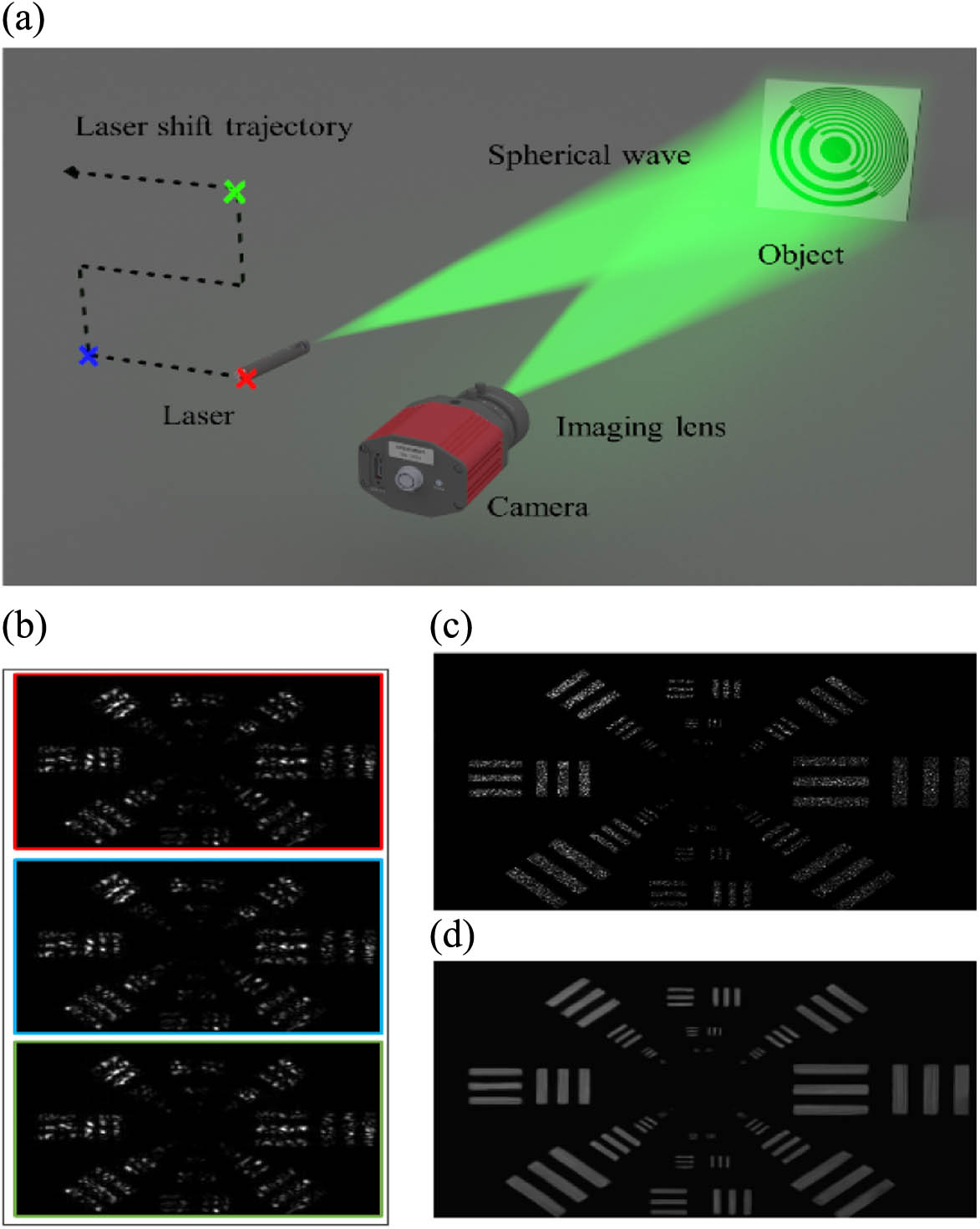
    Fig. 1. (a) Proposed scheme. The object is illuminated by a divergent laser beam to increase the FOV. The scattering from the object is recorded by the sensor via an imaging lens. As the numerical aperture of the imaging system is fixed, a limited resolution image is obtained on the sensor plane. (b) FP raw images. By shifting the laser source with an x-y moving stage, a sequence of raw images is captured. An example of a raw image is blurred and degraded by speckles. Using the captured image sequence, the super-resolution reconstruction can be achieved with the proposed method. The FP reconstruction in (c) reduces the speckle size and improves the resolution. A speckle denoising algorithm is further performed to improve the quality of the reconstruction, and its denoising image is shown in (d).
    Comparisons between two typical remote images via FP. (a), (b) Camera scanning and its FOV reduction. (c), (d) Laser scanning and its FOV reduction.
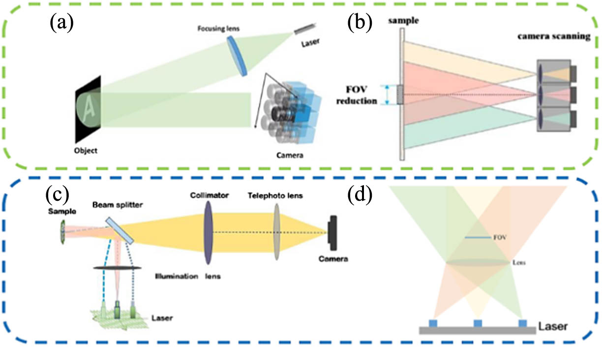
    Fig. 2. Comparisons between two typical remote images via FP. (a), (b) Camera scanning and its FOV reduction. (c), (d) Laser scanning and its FOV reduction.
    Comparisons among three kinds of illumination schemes for remote imaging via FP. (a) Convergent light illumination. (b) Quasi-plane wave illumination. (c) Divergent light illumination. For simplicity, the coordinate of the object’s transverse plane is x. The laser is located at xs, and its distance to the object’s center is zs. The object distance zo and the image distance zI satisfy the lens law of geometrical optics: 1/f=1/zo+1/zI, where f is the focal length.
    Fig. 3. Comparisons among three kinds of illumination schemes for remote imaging via FP. (a) Convergent light illumination. (b) Quasi-plane wave illumination. (c) Divergent light illumination. For simplicity, the coordinate of the object’s transverse plane is x. The laser is located at xs, and its distance to the object’s center is zs. The object distance zo and the image distance zI satisfy the lens law of geometrical optics: 1/f=1/zo+1/zI, where f is the focal length.
    Proposed despeckle algorithm with flow chart (on the left) and despeckle simulation (on the right). (b) The speckle image is simulated from the (a) ground truth based on the negative exponential distribution. (d) The proposed method presents more favorable result than the (c) BM3D algorithm in terms of both the quantitative SSIM and PSNR metrics and the visual quality.
    Fig. 4. Proposed despeckle algorithm with flow chart (on the left) and despeckle simulation (on the right). (b) The speckle image is simulated from the (a) ground truth based on the negative exponential distribution. (d) The proposed method presents more favorable result than the (c) BM3D algorithm in terms of both the quantitative SSIM and PSNR metrics and the visual quality.
    Comparison of FP-based synthetic aperture imaging with different phase terms. The resolution target is used as the amplitude. (a) Results when the phase term is zero. (b) Results when the phase term is quadratic phase. (c) Results when the phase term is a mixture of quadratic phase and random phase. (a-1)–(c-1) Fourier spectrum. (a-2)–(c-2) Raw image with small aperture. (a-3)–(c-3) Synthetic aperture.
    Fig. 5. Comparison of FP-based synthetic aperture imaging with different phase terms. The resolution target is used as the amplitude. (a) Results when the phase term is zero. (b) Results when the phase term is quadratic phase. (c) Results when the phase term is a mixture of quadratic phase and random phase. (a-1)–(c-1) Fourier spectrum. (a-2)–(c-2) Raw image with small aperture. (a-3)–(c-3) Synthetic aperture.
    (a) Experimental setup: 10 m standoff-distance super-resolution coherent imaging over the landscape painting. The target and the imaging setup are shown in (a-1) and (a-2), respectively. Note that the experiment is performed in the dark environment at night with the light off. The imaging area is about 1 m×0.7 m marked in blue box. (b) The raw image shows low resolution and strong speckles. After the six times super-resolution with FP, the (c) reconstructed image significantly improves the resolution and reduces the speckle size. Further despeckle processing is performed on the FP reconstructed image, and the (d) despeckled image is smooth after reducing the intensity variation in the speckle regions. The brightness of (b-2), (c-2), and (d-2) is adjusted for better visualization. (a-1) Target. (a-2) Imaging setup. (b) One example of camera output. (c) Reconstruction. (d) Reconstruction with denoising.
    Fig. 6. (a) Experimental setup: 10 m standoff-distance super-resolution coherent imaging over the landscape painting. The target and the imaging setup are shown in (a-1) and (a-2), respectively. Note that the experiment is performed in the dark environment at night with the light off. The imaging area is about 1  m×0.7  m marked in blue box. (b) The raw image shows low resolution and strong speckles. After the six times super-resolution with FP, the (c) reconstructed image significantly improves the resolution and reduces the speckle size. Further despeckle processing is performed on the FP reconstructed image, and the (d) despeckled image is smooth after reducing the intensity variation in the speckle regions. The brightness of (b-2), (c-2), and (d-2) is adjusted for better visualization. (a-1) Target. (a-2) Imaging setup. (b) One example of camera output. (c) Reconstruction. (d) Reconstruction with denoising.
    10 m standoff-distance super-resolution coherent imaging over the resolution target. (a) Ground truth of self-designed resolution target containing different resolution charts, where the bottom right target will further be used for qualitative analysis of resolution in Fig. 9. (b) Raw image captured by the imaging system. (c) Reconstructed image with FP super-resolution. (d) Despeckled image from the FP reconstructed results. (a-1), (a-2), (b-1), (b-2), (c-1), (c-2), (d-1), (d-2) are zoomed images from (a), (b), (c), and (d). The brightness of (b), (c), and (d) is adjusted for better visualization.
    Fig. 7. 10 m standoff-distance super-resolution coherent imaging over the resolution target. (a) Ground truth of self-designed resolution target containing different resolution charts, where the bottom right target will further be used for qualitative analysis of resolution in Fig. 9. (b) Raw image captured by the imaging system. (c) Reconstructed image with FP super-resolution. (d) Despeckled image from the FP reconstructed results. (a-1), (a-2), (b-1), (b-2), (c-1), (c-2), (d-1), (d-2) are zoomed images from (a), (b), (c), and (d). The brightness of (b), (c), and (d) is adjusted for better visualization.
    USAF resolution target is used to characterize the resolution under different synthetic apertures with FP. (a) Raw image and examples of reconstructed images of SA 10 mm, SA 18 mm, and SA 35 mm. (b) Magnified regions of various bar groups in (a). The blue dashed line demarcates resolvable features. Features below this line are resolvable. (c) Contrast plots for the reconstructed images with SA=18 mm and SA=35 mm. (d) Resolution is inversely proportional to the size of the synthetic aperture. The stars denote the limiting resolution by visually inspecting the recovered images with FP-based super-resolution and despeckle processing under various SA. We observe that the visually determined resolution agrees with the proposed limit [Eq. (1)] for coherent imaging. Moreover, the proposed despeckle procedure does not degrade the resolution, and it helps to discriminate the bars by reducing the speckle variation. The brightness of (a) and (b) is adjusted for better visualization.
    Fig. 8. USAF resolution target is used to characterize the resolution under different synthetic apertures with FP. (a) Raw image and examples of reconstructed images of SA 10 mm, SA 18 mm, and SA 35 mm. (b) Magnified regions of various bar groups in (a). The blue dashed line demarcates resolvable features. Features below this line are resolvable. (c) Contrast plots for the reconstructed images with SA=18  mm and SA=35  mm. (d) Resolution is inversely proportional to the size of the synthetic aperture. The stars denote the limiting resolution by visually inspecting the recovered images with FP-based super-resolution and despeckle processing under various SA. We observe that the visually determined resolution agrees with the proposed limit [Eq. (1)] for coherent imaging. Moreover, the proposed despeckle procedure does not degrade the resolution, and it helps to discriminate the bars by reducing the speckle variation. The brightness of (a) and (b) is adjusted for better visualization.
    Resolution analysis of 10 m super-resolution coherent imaging. (a) Zoomed images of resolution bars from the right bottom of Figs. 7(a)–7(d). (b) Close ups of resolution bars with different resolutions. The resolution of the raw image is 0.25 lp/mm. After the FP reconstruction and despeckle processing, the resolution is increased to 1.4 lp/mm. The brightness of (a) and (b) is adjusted for better visualization.
    Fig. 9. Resolution analysis of 10 m super-resolution coherent imaging. (a) Zoomed images of resolution bars from the right bottom of Figs. 7(a)–7(d). (b) Close ups of resolution bars with different resolutions. The resolution of the raw image is 0.25 lp/mm. After the FP reconstruction and despeckle processing, the resolution is increased to 1.4 lp/mm. The brightness of (a) and (b) is adjusted for better visualization.
    Comparison of the SAVI and the proposed scheme. To make a fair comparison, similar parameters are used for the setups of both schemes. The camera with 2.34 mm aperture is placed 1 m away from the object. A grid of 26×26 images is captured with 78% overlap ratio to achieve a synthetic aperture of size 14.84 mm. (a)–(c) Low-res image, reconstructed image, and denoised image with the proposed method. (d)–(f) Low-res image, reconstructed image, and denoised image of SAVI scheme.
    Fig. 10. Comparison of the SAVI and the proposed scheme. To make a fair comparison, similar parameters are used for the setups of both schemes. The camera with 2.34 mm aperture is placed 1 m away from the object. A grid of 26×26 images is captured with 78% overlap ratio to achieve a synthetic aperture of size 14.84 mm. (a)–(c) Low-res image, reconstructed image, and denoised image with the proposed method. (d)–(f) Low-res image, reconstructed image, and denoised image of SAVI scheme.
    Superimposed intensity of two coherent points in the case of phase differences φ0=0, π/2, and π. Two points are angularly displaced with (a) Δθ=1.22λ/D and (b) Δθ=1.60λ/D. Superimposing is simulated using Eqs. (A1) and (A2). When φ0=π, the two points are always resolvable. And for the worst case φ0=0, two points are just resolvable when Δθ=1.60λ/D.
    Fig. 11. Superimposed intensity of two coherent points in the case of phase differences φ0=0, π/2, and π. Two points are angularly displaced with (a) Δθ=1.22λ/D and (b) Δθ=1.60λ/D. Superimposing is simulated using Eqs. (A1) and (A2). When φ0=π, the two points are always resolvable. And for the worst case φ0=0, two points are just resolvable when Δθ=1.60λ/D.
    Plot of central-to-peak ratio versus angular displacement Δθ in the case of ϕ0=0.
    Fig. 12. Plot of central-to-peak ratio versus angular displacement Δθ in the case of ϕ0=0.
    Simulated speckle image of double splits under various angular displacements between two splits. (a) Δθ=1.40λ/D, (b) Δθ=1.60λ/D, and (c) Δθ=1.80λ/D.
    Fig. 13. Simulated speckle image of double splits under various angular displacements between two splits. (a) Δθ=1.40λ/D, (b) Δθ=1.60λ/D, and (c) Δθ=1.80λ/D.
    Gaussian fitting for the probability distribution of nlog and ntran. (a) Fitting results of p(nlog) and (b) fitting results of p(ntran).
    Fig. 14. Gaussian fitting for the probability distribution of nlog and ntran. (a) Fitting results of p(nlog) and (b) fitting results of p(ntran).
    Zhiming Tian, Ming Zhao, Dong Yang, Sen Wang, An Pan. Optical remote imaging via Fourier ptychography[J]. Photonics Research, 2023, 11(12): 2072
    Download Citation