Optical remote imaging is one of the important means and technical supplement of remote sensing. Improving the resolution of space cameras has been unremittingly explored in the field of high-resolution remote sensing. The angular resolution is defined as 1.22λ/D, where λ is the center wavelength, and D denotes the size of the imaging aperture [1]. According to the formula, increasing the aperture of a space camera, especially the main mirror, is the most direct way to improve spatial resolution and extend the field of view (FOV). However, it imposes geometric aberrations to the optical system; thus more optical surfaces are required to optimize the aberrations in turn, which brings a series of problems such as a larger volume of space cameras and increased cost and launch risk [2]. Therefore, the aperture of a single mirror in space cameras based on the traditional incoherent imaging system cannot be increased infinitely and is also limited by manufacturing techniques.

A passive optical synthetic aperture camera can bypass the manufacturing of large-aperture mirrors, but it must ensure the confocal and cophase between sub-apertures. For example, the six sub-apertures in Golay6 must achieve strict confocal and cophase with an accuracy of up to λ/10 to meet the imaging requirements [3,4], which requires extremely high performance of phase detection and posture control. Moreover, the stability of the platform is demanding, which makes it tough to be widely applied in engineering.

Synthetic aperture radar (SAR) is an active high-resolution radar technology that can directly measure the complex amplitude wave field of sub-apertures through an antenna with a temporal resolution of picoseconds, and then stitch this sub-aperture information in the frequency domain to obtain a virtual large aperture with high resolution [5]. Efforts have been made to extend the concept of synthetic apertures to the near-infrared band [6–8]. According to the spatial resolution formula, the imaging resolution can be further improved if realizing synthetic apertures in the visible range of light. However, the optical band is four to five orders of magnitude higher than the microwave frequency. Compared with antennas, an optical detector needs to record the complex amplitude wave field at the level of femtoseconds, which is far beyond the ability of modern imaging devices.

Fourier ptychographic microscopy (FPM) is a promising computational imaging technique invented by Zheng et al. in 2013 [9]. It is named after ptychography, which was proposed by Rodenburg and Faulkner in 2004 [10]. FPM uses coherent illumination to produce a relative shift between the aperture and object’s spectrum, and then captures a set of low-resolution images corresponding to different sections of the Fourier spectrum using a small-aperture lens. Fusing the spectrum of these low-resolution images in the Fourier domain can reconstruct a high-resolution image corresponding to a larger synthetic aperture. It breaks through the trade-off between high resolution and large FOV in traditional optical imaging with a combination of synthetic aperture and phase retrieval [11,12]. At the same time, it recovers aberrations of the optical system, and thus realizes digital compensation of aberrations for the full FOV [13]. Currently, FPM has been proved not only to be a powerful tool to solve the constraints of FOV and resolution, but also a paradigm to address a series of trade-off problems, such as the intrinsic trade-off between angular resolution and spatial resolution in the field of light field microscopy [14].

In 2014, Dong et al. [15] first reported a conceptual experiment that extended the application scenario of FPM from micro to macro imaging, opening the possibility of FP technology in industrial inspection or remote imaging. This has attracted much attention, and a series of related work can be referred to Refs. [16–20]. Notably, Holloway et al. [5] reported the FP-based optical synthetic aperture visible imaging, termed SAVI. In 2017, they further improved the theory and built a long-range reflective FP imaging device [21]. The imaging distance was extended from 0.7 to 1.5 m, and the imaging resolution was improved by six times. In the implementation of SAVI, two fundamental modifications are required to adapt previous FPM to long-distance imaging. First, as the distance is increased by orders of magnitude, a highly flexible setup based on reflective illumination and camera scanning was presented. Second, previous works relied on smooth targets. While imaging everyday objects with rough surfaces that scatter incident light in random directions, denoise processing is needed to address the resultant speckle. However, the FOV is always changing slightly due to the camera scanning scheme, and the effective FOV that can be recovered eventually is only the area where all sub-apertures overlap, so the method has low utilization of FOV. In 2019, we reported a coherent synthetic aperture imaging method based on laser multi-angle illumination [22], called CSAI. The resolution is improved by 4.5 times at the FOV of 12.4 mm. Despite these efforts [21–26], there is still an important scientific problem and two big challenges that need to be addressed. First, the multi-angle coherent model of FP would be destroyed by diffuse objects or atmosphere; thus whether the FP model can improve resolution or suppress speckle is unclear. Second, the imaging distance and the size of FOV are limited since the illumination of convergent light requires extra mirrors in the optical path, which greatly hinders the widespread application. Third, such active illumination of FP requires a dark room and a high-power laser, which is susceptible to stray light and speckle noise.

In this paper, we report an FP imaging scheme for long-range and larger FOV reflective imaging by employing a divergent spherical optical wave for illumination and camera scanning. The divergent spherical wave in our scheme can increase the FOV of illumination and break the limitation of FOV with the convergent optical wave. We provided rigorous theoretical analysis to explain the generation of speckles, which differs from traditional FPM implementations with quasi-plane wave illumination. In our reflective FP scheme, the random phase of the object, coming from its microscopic rough surface variation, will be mixed with a spherical wave so that the captured images are manifested as speckles. As both resolution and speckle size are inversely proportional to aperture size, we demonstrated that by creating a synthetic aperture, our FP imaging scheme is able to reduce speckle size and improve resolution. We analyzed the limit resolution of coherent imaging with speckles based on the Rayleigh criterion, and quantitatively validated the conclusion on our experimental platform, which can be vital for predicting and evaluating the performance of practical coherent imaging systems. To further remove speckles in reconstruction, a despeckle algorithm was presented based on the negative exponential distribution, and we realized PNSR values up to around 25–30 dB in simulations. We experimentally performed a 10 m stand-off FP imaging over an object of size ∼1m×0.7m with a synthetic aperture of 31 mm. The imaging distance and FOV have increased by orders of magnitude compared with the SAVI method. It is noted that our proposed method has the capability for further scaling to a longer range.

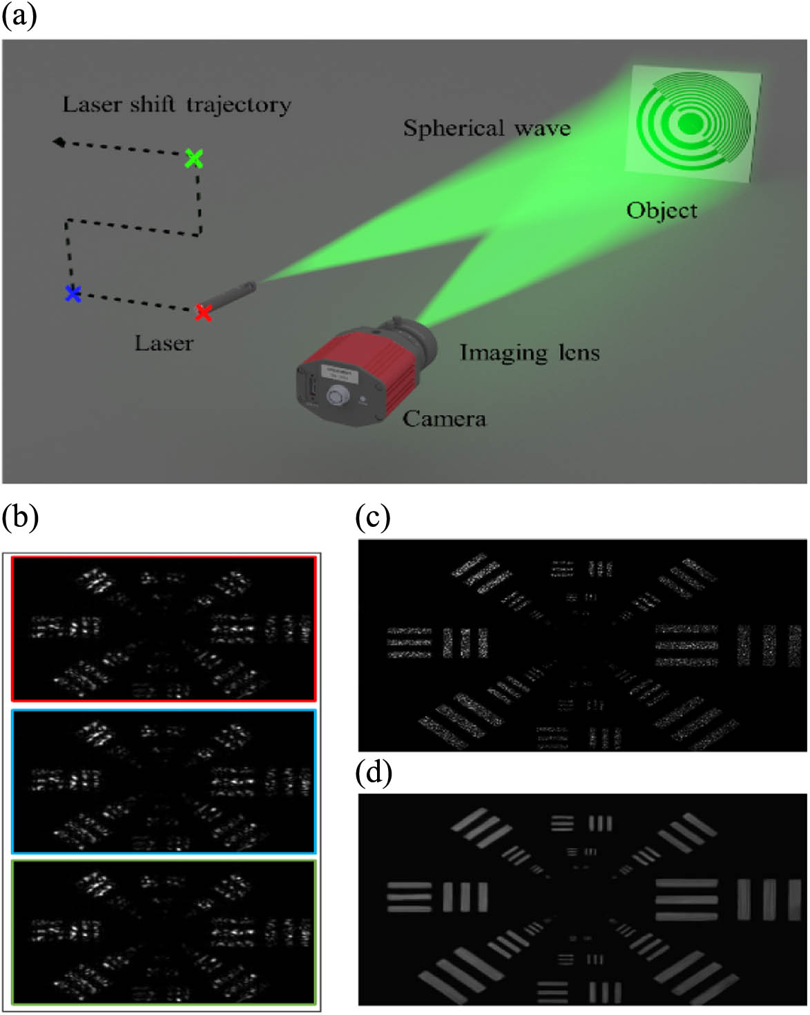
The configuration of our proposed FP imaging system is shown in Fig. 1(a). A divergent spherical wavefront produced by a laser source illuminates the diffuse object, and the reflected light from the object is then captured by a camera. The laser is moved to illuminate the object from different angles, and a sequence of raw images is recorded accordingly as shown in Fig. 1(b). The raw captured image is blurred and degraded due to the influence of large speckles. An image with a synthetic aperture can be reconstructed from these raw images via FP reconstruction. By creating a synthetic aperture, the FP reconstructed image greatly reduces the speckle size and improves the resolution as shown in Fig. 1(c). A speckle denoising algorithm is further operated to improve the quality of the reconstruction as shown in Fig. 1(d).

There are generally two ways to realize relative spectrum shifting in FP imaging. The camera scanning scheme [Fig. 2(a)] is based on the theory that far-field diffraction corresponds to Fourier transform mathematically. Unfortunately, in order to achieve far-field diffraction, the size of the camera lens should be extremely small. For a 10 m distance imaging scenario, the maximum diameter of the camera lens is only 1.6 mm, which is much smaller than what we commonly use. In addition, the scanning of the camera produces a varying FOV and causes a limited FOV in the effective area, as shown in Fig. 2(b).

Laser scanning is another way widely employed in FP imaging, which can basically be classified into three types, as shown in Fig. 3. The illumination of convergent light [Fig. 3(a)] has been utilized in SAVI, and quasi-plane wave illumination [Fig. 3(b)] is quite common in the field of FPM. The two schemes also suffer from a limited FOV as convergence or collimating mirrors are used in the design of the optical path. Meanwhile, the shifting light source illuminates the object from different angles, which implies that the light wave should be generated to cover the whole object’s area. Therefore, they are quite impractical for the case of macroscopic imaging with long distances (e.g., in remote sensing). For the illumination of divergent light, as shown in Fig. 3(c), imaging FOV and distance can both be greatly increased since no extra mirrors are required. The eventual imaging distance is only related to energy intensity and environmental disturbance. This illumination pattern is what we adopted, and the corresponding forward model will be established in the following section, Section 2.B.

As shown in Fig. 3(c), the laser source provides a divergent beam to illuminate the object. We can model the wavefront in front of the object as a spherical wave S(x), which is given by $$\begin{gathered} S(x)≈exp(ik2zs(x−xs)2) \\ =CsQs(x)Ls(x), \end{gathered}$$(1)where Cs=exp(ikxs·xs/2zs) is the constant phase term irrelevant to the object plane x, and Ls(x)=exp(−ikx·xs/zs) and Qs(x)=exp(ikx·x/2zs) are the linear phase term and the quadratic phase term. The illumination is transmitted to the object, and part of reflection is directed to the camera. The field Es(x) immediately after the object is $$\begin{gathered} Es(x)=S(x)O(x) \\ =S(x)A(x)exp(ikθo(x)) \\ =CsA(x)exp(ikθo(x))Qs(x)Ls(x), \end{gathered}$$(2)where A(x) is the amplitude of the object, and θo(x) is the object’s random phase that comes from the random height fluctuation of the surface. The object field Es(x) travels to the camera lens over a distance zo, and then propagates an imaging distance zI to the sensor plane. According to the lens law of geometrical optics (1/f=1/zo+1/zI), the intensity image captured by the sensor is given by $$\begin{gathered} I(ξ)=|F−1{F{Es(x)Qo(x)}×P(u)}|2 \\ =|F−1{F{A(x)eikθo(x)Qs(x)Qo(x)Ls(x)}×P(u)}|2, \end{gathered}$$(3)where Qo(x)=exp(ikx·x/2zo) is the quadratic phase term from the object to the lens. P(u) is the pupil function of the lens, and the vector u is the frequency coordinate. For an aberration-free optical system, the pupil function is given by P(u)={1|u|<D/20else.(4)We define the dummy object as $$\begin{gathered} ω(x)=A(x)exp(ikθo(x))Qs(x)Qo(x) \\ =A(x)exp(ik(1zs+1zo)x·x+iθo(x)). \end{gathered}$$(5)Substituting Eq. (5) into Eq. (3), the FP forward model under a spherical wave is given by $$\begin{gathered} Is(ξ)=|F−1{F{ω(x)Ls(x)}×P(u)}|2 \\ =|F−1{Ω(u−us)P(u)}|2, \end{gathered}$$(6)where Ω(u) is the Fourier spectrum of the dummy object ω(x), and us=kxs/zs is the relative spectrum shift produced by the linear phase Ls(x) of the light source. Moving the light source varies the linear phase Ls(x), and thus shifts the dummy object’s spectrum Ω(u) relative to the lens aperture. In this way, the FP-type dataset can be captured.

Using phase retrieval algorithms, FP allows the recovery of missing phase with the constraint from the overlaps between the sub-aperture spectrum. Although extensive works have been contributed to solving the FP phase retrieval problem [13,27–30], the alternating projection (AP) method is still the stable and widely used option. The concept of AP originated from the Gerchberg–Saxton (GS) algorithm, where the magnitude constraints from the measured images are imposed to the field estimate in the image domain.

In the mth iteration, the current estimates of the object and the pupil function are denoted as Ω(m)(u) and P(m)(u). For the sth image Is(ξ), the sub-spectrum estimate Ψs(m)(u) is inversely Fourier transformed to form the estimate of the field, denoted as ϕs(m)(ξ)=F−1{Ψs(m)(u)}. We impose the magnitude constraint to ϕs(m)(ξ) as ϕs(m+1)(ξ)=Is(ξ)ϕs(m)(ξ)|ϕs(m)(ξ)|.(7)We can then obtain the updated sub-spectrum estimate as Ψs(m+1)(u)=F{ϕs(m+1)(ξ)}. Ω(u) and P(u) are then updated according to the gradient descent scheme as Ω(m+1)(u)=Ω(m)(u)+conj(P(m)(u+us))max2(|P(m)(u+us)|)(Ψs(m+1)(u+us)−Ψs(m)(u+us)),(8)$$\begin{gathered} P(m+1)(u)=P(m)(u)+conj(Ω(m)(u−us))max2(|Ω(m)(u−us)|) \\ ×(Ψs(m+1)(u)−Ψs(m)(u)). \end{gathered}$$(9)The initial estimate of the pupil function P(u) is defined to be an ideal circular aperture from Eq. (4). The Fourier transform of the average of all captured intensity images is chosen to initialize Ω(u), which helps to suppress speckle in images.

Speckle is not real noise in a conventional sense. Since the random phase distorts the intensity field, the seeming randomness of the speckle intensity manifests as “noise.” The probability of the speckle intensity I follows the negative exponential distribution [31] p(I)∝exp(−I/μ), where μ is the uncorrupted intensity represented as the mean intensity. It is straightforward to establish a multiplicative noise model I=μ×n, where n is the multiplicative speckle noise and satisfies p(n)∝exp(−n). By taking the logarithm of the multiplicative noise model, it is transformed into the additive noise model Ilog=ln(I)=ln(μ)+ln(n)=μlog+nlog.(10)The probability distribution of nlog is non-Gaussian, so the classical Gaussian-based denoising algorithms are less effective on the speckle noise.

Here, we propose a novel speckle denoising algorithm; refer to Appendix B for the specific deduction. The flowchart of the algorithm is shown in Fig. 4. We first take the logarithm of the speckle image I as Ilog=ln(I). The logarithmic speckle noise is estimated as n^log=Ilog−De(Ilog), where De(·) is the BM3D denoising operation [32]. n^log is then transformed according to n^tran=f(n^log), where f(v) is the transformation function defined by f(v)=v when v≥0 and f(v)=−−v when v<0. The new noisy image is constructed by I^tran=De(ylog)+n^tran. We can obtain the denoised logarithmic image as μ^log=De(I^tran). Finally, FP reconstruction is operated and a denoised reconstructed image can be obtained.

Figures 4(a)–4(d) show the simulation result of our speckle denoising algorithm and its comparison with the BM3D algorithm. A cameraman picture is chosen as the ground truth, and the speckles are produced based on the negative exponential distribution. We select the peak signal-to-noise ratio (PSNR) and structural similarity (SSIM) as the criteria to evaluate despeckling performance. It can be seen that our algorithm provides much cleaner background information, presenting a more powerful ability to eliminate the effect of speckle.

First, we conducted simulations to visualize and explain FP reconstruction of the object, where a resolution target is used as the amplitude, and three kinds of phase terms are considered. When illuminated by plane waves, the object contains no phase term. As shown in Fig. 5(a-1), the spectrum follows a nicely structured pattern with a peak at the DC component and decaying magnitudes for high spatial frequency. The raw images contain brightfield images and darkfield images, corresponding to the DC component and high frequency, respectively. Stitching up the spectrum from these raw images can finally produce a high-resolution image. The quadratic phase term is the case where a spherical wave is used to illuminate transmissive objects. One obvious difference with the no-phase case is that each raw image contains a brightfield part and a darkfield part, as shown in Fig. 5(b-2), since the quadratic phase term introduces optical waves with higher incident angles exceeding the numerical aperture. Also, the FOV expands along with the improved resolution [Fig. 5(b-3)].

Figure 5(c) shows our case where the phase term is the mixture of random phase and quadratic phase. As seen from Eq. (5), the phase of dummy objects contains two parts: quadratic phase from the optical path and imaging lens and random phase of the rough surface. The spectrum does not exhibit any meaningful structure since the random phase dominates the quadratic phase. As shown in Fig. 5(c-2), the raw images of the dummy object are distributed with speckles, which degrades the image quality. By creating a large synthetic aperture, we can reduce the speckle size and recover the high-resolution image of the dummy object as shown in Fig. 5(c-3). In conclusion, FP reconstruction enables high-fidelity recovery of phase information, even when the phase fluctuates significantly as random phase. Although the amplitude is of the most concern in coherent imaging, the phase term will have a profound impact on the image when the aperture is limited.

We performed a 10 m standoff-distance experiment to demonstrate the performance of our scheme. The imaging distance is around 10 times that of the state-of-the-art method in SAVI [21]. The experimental setup is shown in Fig. 6(a). The divergent beam is produced using a 532 nm single-mode laser source and a plano–concave lens (focal length of −10mm). We employ a lens with 75 mm focal length and 5 mm aperture for imaging, and then record the raw images with an image sensor (IMX178, 2048×3056pixels, 2.4 μm pixel pitch). In addition, a linear polarizer is placed before the camera to filter out the noninterference light. We selected a large landscape painting as the object, and part of the painting (∼1m×0.7m) is imaged by our system. A 2D translation stage (Zolix, PSA050-11-X) is used to shift the laser source with the step size of 0.875 mm, resulting in an overlapping rate of 82.5%. Here, the camera is facing the object directly, and the scanning plane of the light source is perpendicular to the camera’s normal direction. A grid of 31×31 low-resolution images is collected, and the maximum synthetic aperture is 31 mm, which is six times larger than the lens’ aperture.

A single capture from the imaging system is shown in Fig. 6(b). Due to the limitation of the aperture, the raw image exhibits significant blur and diffraction. As the surface of the painting is rough, severe speckles can be observed, which further degrade the image quality. As seen in Fig. 6(c), the reconstructed image can provide much higher resolution and the size of speckles is decreased compared with the raw data. For example, we can clearly observe the mild structure on the building in Fig. 6(c1) and leaf patterns in Fig. 6(c2), which are not resolvable in the raw captures. After applying the proposed speckle denoising algorithm, the speckles are smoothed and removed, resulting in better visual quality as shown in Fig. 6(d).

Next, we performed the experiment on a self-designed resolution target (42cm×29.7cm) using the same experimental setup. The target contains several types of commonly used resolution charts as shown in Fig. 7(a). A grid of 27×27 low-resolution images is collected, and the maximum synthetic aperture is 27.75 mm. The raw image captured by the imaging system is shown in Fig. 7(b), which is distributed with large speckles. After the FP reconstruction, the image resolution is greatly improved with a smaller size of speckles. The denoising algorithm effectively removes the effect of speckles, improving the image contrast while retaining the same resolution improvement as traditional FP algorithms. The results presented above are based on a qualitative analysis of resolution; we will further provide the related quantitative performance in the consequent section.

The Rayleigh criterion has been widely used for resolution estimation in incoherent imaging. Two incoherent point sources apart with the Rayleigh limit can just be resolved. It becomes complex for coherent imaging as the interference intensity is phase dependent although the complex field is linear [33,34]. In this case, two coherent point sources with the same phase will not be resolved. However, they become fully resolved when the two sources have a phase difference of π.

For reflective coherent imaging, the random phase of a rough surface will produce speckles, which degrade image quality and resolution. A conservative way to define the resolution limit is to consider the worst case. Considering two point sources with the same phase, it is easy to obtain the profile of the superimposed intensity. Theoretically, it can be calculated from the superimposed image that when the central dip’s intensity is 81% of maximum intensity on either side, the angular distance of two points is 1.60λ/D (see Appendix A). Thus, the Rayleigh limit for coherent imaging under speckle is defined as R=1.60λD,(11)where λ is the wavelength, and D is the diameter of the imaging lens.

To investigate the resolution performance of our method, we imaged a negative USAF target with white paint sprayed to the chrome surface, as in the work of SAVI [21]. The imaging distance is reduced to 1 m due to the small size of the target (18mm×18mm). The target is imaged through the back of a glass plate to retain the high-resolution features. The laser source is translated with the stepsize of 1 mm, resulting in an overlapping rate of 80%. A grid of 31×31 low-resolution images is collected, and the maximum synthetic aperture is 35 mm.

The reconstruction results with SA of 10 mm, 18 mm, and 35 mm are presented in Fig. 8(a). It can be seen that an increased synthetic aperture leads to higher resolution and smaller speckle size. We then process the reconstructed results with the speckle denoising algorithm. The imaging quality further improves with the removal of speckle patterns. Figure 8(b) shows the close-up reconstructed images of four typical patterns in the target. The blue dashed line demarcates resolvable features, and the features below this line can be clearly identified. The contrast metric is selected as the criterion to evaluate the resolution performance, which is given by C=W−BW+B,(12)where W and B are average intensity values for three white and two black bars of the pattern, respectively. The area of bars is manually located using a high-resolution USAF image and then scaled to the correct size for each tested image. Figure 8(c) plots the contrast metric for reconstructed images with SA=18mm and SA=35mm. Obviously, the contrast is improved with the increase of synthetic aperture.

Moreover, we set a contrast threshold as 0.1 to determine the limit resolution of the reconstructed images, since the value of the contrast metric is around 0.1 for the Rayleigh criteria (C=(1−0.81)/(1+0.81)≈0.1). The minimum resolvable line width of various SA is then determined, and marked by red stars in Fig. 8(d). We can see that the experimental resolution limit roughly agrees with the curve of theoretical values.

Using the resolution bars from the right bottom of Fig. 7, we quantitatively demonstrate the resolution performance of our scheme, and the results are shown in Fig. 9. The theoretical minimum resolvable line width is 1.7 mm. As can be seen in the raw image of Fig. 9(b), the bars can be resolvable when the line width is 2 mm. FP reconstruction improves the resolution to 0.357 mm line width, which is at least 4.7 times smaller compared with the raw image.

We experimentally duplicated a 1 m standoff-distance SAVI setup to validate the FOV expansion of our method compared with the camera scanning scheme of SAVI. A convex lens (diameter: 2 inches, focal length: 300 mm) is inserted between the laser source and the target to compensate for the quadratic phase. As illustrated in Fig. 3(a), the illumination is converged after the lens, and thus a light spot will appear on the target plane. The spot size has been confined by the practical size of the lens, which leads to the limited FOV of SAVI. The camera is mounted on the translation stage and moved to realize spectrum shifting. The distance between adjacent positions of the camera is 0.5 mm to ensure an overlapping rate of 78%. A grid of 26×26 images is captured to produce a synthetic aperture of 14.84 mm. The experimental results of SAVI are shown in Figs. 10(d)–10(f). To make a fair comparison, we keep the configuration of the setup exactly the same as SAVI. We only replace the compensation lens in SAVI with a plano–concave lens (diameter: 6 mm, focal length: −6mm) to produce a divergent beam. The experimental results of our method are shown in Figs. 10(a)–10(c). As we can see, our method demonstrates a significantly improved FOV (around six times) compared with SAVI.

We demonstrated a reflective long-range FP imaging scheme, which allows synthetic aperture imaging with large FOV. Existing methods, which image diffuse reflective objects with optically rough surfaces, lack an underlying physical explanation for principles. We have established a forward model with rigorous deduction to prove that FP can be used for diffuse reflective objects, rather than simply suppressing speckle. Our 10 m standoff-distance experiment realized a theoretical synthetic aperture with ∼1mm2 FOV. The imaging distance and FOV have increased by orders of magnitude compared with SAVI method. We performed the proposed speckle denoising algorithm on simulated data, and the PSNR value can be improved up to around 25–30 dB. In addition, we analyzed the limit resolution of coherent imaging with speckles based on the Rayleigh criterion, and quantitatively validated the conclusion on our experimental platform, which can be vital for predicting and evaluating the performance of practical coherent imaging systems (e.g., laser imaging, laser display).

An important issue following naturally would be how our scheme can be extended to more complex application scenarios. When imaging at a much longer distance (like 1 km), one main challenge for our scheme lies in the atmospheric turbulence [35], which might introduce unstable and fluctuated distortion to illumination and reflection wavefronts. The distortion on an illumination wavefront should present a limited effect since it can be overwhelmed by the random phase as the forward model discussed in Section 2.B. The distortion on the reflection wavefront, on the other hand, can be problematic for long-range imaging like astronomy imaging. Actually, the turbulence can be regarded as the wavefront error in the pupil function [36]. As FP reconstruction allows correction of aberrations, it becomes possible to reconstruct the pupil function with a turbulent wavefront. To tackle the space-variant wavefront distortion, FP reconstruction can be performed targeted at small image patches where the distortion can be approximated to be space-invariant. In addition, it can be feasible to minimize the capture time to freeze the distorted wavefront by using the camera array or laser array, that is, to reduce the impact of atmospheric disturbance by improving data collection efficiency. The effect of stray light might be another problem to be solved, which is well worthy of study and discussion in future work. Possible solutions include filtering out light with certain wavelengths or using a lens hood to suppress stray light when necessary.

References

[1] J. W. Goodman. Introduction to Fourier Optics(2005).