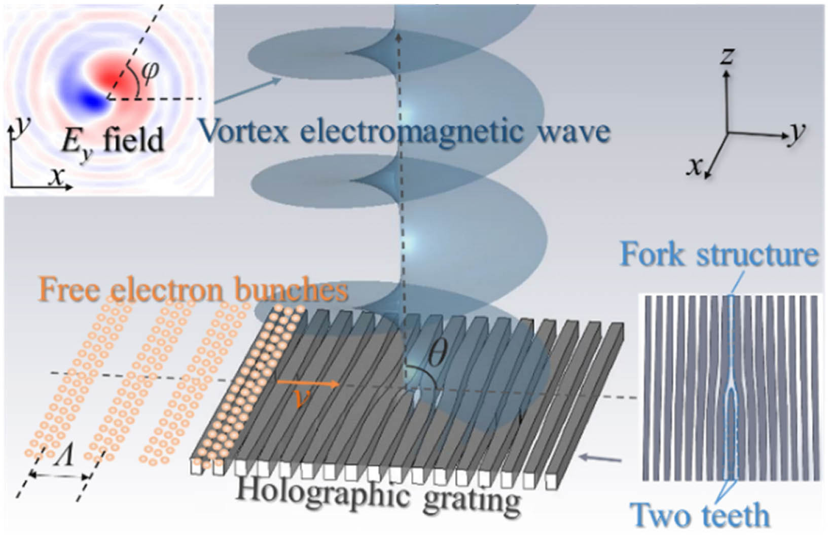
Fig. 1. Schematic diagram of generating vortex Smith–Purcell radiation (with a TC of l=1 for example) with free-electron bunches and holographic grating. The free electrons are periodically bunched in the y direction with pitch Λ much smaller than the radiating wavelength. The velocity of the electron bunches is v. The holographic grating (top view is shown in the inset) is made of metal or dielectrics depending on the frequency of VSPR and has a fork structure with two teeth. When periodic free-electron bunches pass on the holographic grating, an orbital angular momentum (OAM) wave would be emitted at an angle θ with respect to the y axis.

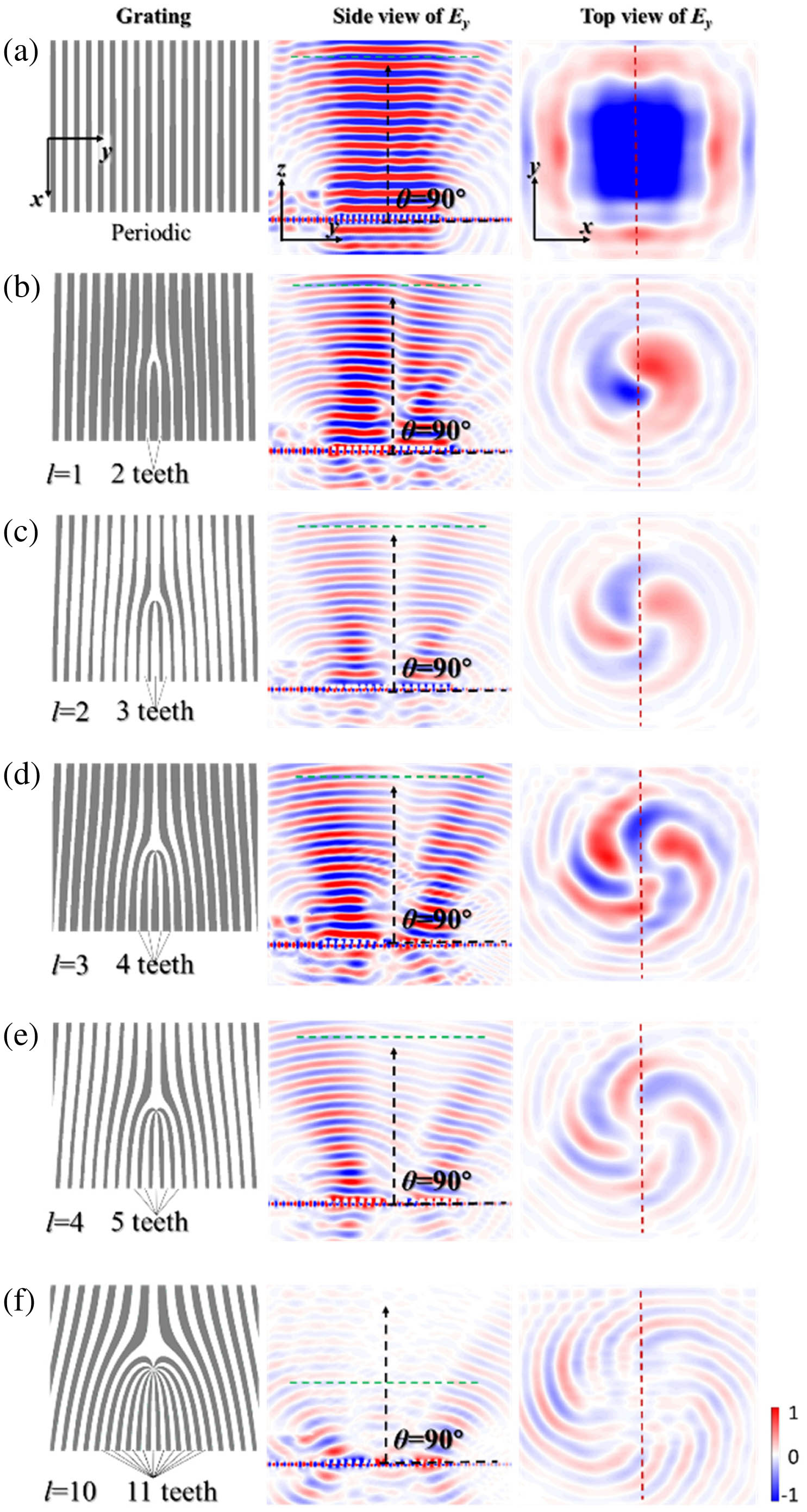
Fig. 2. Simulation of a THz OAM wave with TCs of (a) 0 (traditional SPR from periodic grating), (b) 1, (c) 2, (d) 3, (e) 4, and (f) 10. Left: Top view of the gratings (gray part represents PEC, white part represents vacuum), in which the teeth of the fork structures are marked. Middle: Side view of the Ey field (Ey in the y–z plane, the observation planes are shown as red-dashed lines in the right colomn) of the OAM wave with different TCs. The radiation angle is about 90°, and the vortex wave propagates along the z direction. Right: Top view (the observation planes are shown as green-dashed lines in the middle column) of the Ey field above the grating, which clearly shows the vortex shape and the phase change of l×2π (l=0,1,2,3,4, and 10) with φ varying 2π.

Fig. 3. Simulation of THz VSPR with mixed mode of l=1 and l=2 (ratio of intensity: 0.5:0.5). (a) The holographic grating used in this simulation; (b) side view of the radiation field (Ey in the y–z plane); (c) top view of the radiation field (Ey in the x–y plane). The observation plane is 10 mm away from the holographic grating. (d) Normalized OAM spectrum of the radiated beam, in which the intensity is 0.40 for the l=1 mode and 0.41 for the l=2 mode.

Fig. 4. OAM wave at f=1  THz with l=1 generated by electrons with velocity of (a) v=c/3 (Ek=31.0  keV), (b) v=c/10 (Ek=2.57  keV), (c) v=c/20 (Ek=0.640  keV). Left: The holographic grating for different electron velocities. Middle: Side view of the radiated Ey field (the observation planes are shown as the red-dashed lines in the right colomn). The green rectangles circle the holographic gratings. Right: Top view of the radiated Ey field. The observation planes for the right figures are perpendicular to the z axis (shown as the green-dashed lines in the middle colomn). The field is normalized individually in each figure.

Fig. 5. OAM wave generated by free electrons with bunching frequency of (a) 0.68 THz, (b) 0.6 THz, and (c) 0.43 THz. Left, Ey field in the y–z plane. Right, Ey field of the OAM wave in the observation plane perpendicular to the propagating direction (corresponding to the green dashed line). The corresponding radiation frequency (wavelength) is 1.36 THz (220 μm), 1.2 THz (250 μm), and 0.86 THz (350 μm), which follows the formula raised by Smith and Purcell. The parameters of the holographic grating are the same as those of Fig. 2(c), and the free-electron velocity is v=c/3.

Fig. 6. (a) Schematic of the Huygens construction for conventional SPR with a radiation angle of θ=90°. A train of free-electron bunches passes above a conventional grating. The red and black dashed arc lines represent the wave fronts of the wavelets generated by the electrons in respective color, while the gray ones show the equiphase surfaces of the wavelets corresponding to second-order SPR, which has 2π×N (N=1,2,3…) phase delay compared with the wave front. The blue and orange lines show the equiphase surfaces of the SPR. Three-dimensional schematics of the equiphase surfaces of the conventional SPR are shown below. The distances between each two adjacent equiphase surfaces (namely, wavelength) are λ1 and λ1/2 for the first- and second-order SPR, respectively. (b) Schematic of the equiphase surface of the first- and second-order OAM generated by holographic grating. (c) Second-harmonic OAM wave at frequency of 2 THz. The holographic gratings shown in the inset are the same as those illustrated in the left figures of Fig. 2. The TC of second-harmonic OAM wave is doubled compared with that of fundamental mode.

Fig. 7. OAM wave generated in different frequency regions. The field plotted in each figure is normalized individually. The holographic gratings for different frequencies have similar profile to the left figure in Fig. 2(d), but the scales of the holographic gratings and material permittivity are different, which are shown in Table 1.

Table 1. Parameters of the Simulations in Different Frequency Regions