Single-View Enhanced Cerenkov Luminescence Tomography Based on Sparse Bayesian Learning

Yuqing Hou; Hua Xue; Xin Cao; Haibo Zhang; Xuan Qu; Xiaowei He

doi:10.3788/AOS201737.1217001

Journals >Acta Optica Sinica >Volume 37 >Issue 12 >Page 1217001 > Article

Acta Optica Sinica
Vol. 37, Issue 12, 1217001 (2017)

Single-View Enhanced Cerenkov Luminescence Tomography Based on Sparse Bayesian Learning

Yuqing Hou, Hua Xue, Xin Cao, Haibo Zhang, Xuan Qu, and Xiaowei He^*

Author Affiliations

School of Information and Technology, Northwest University, Xi'an, Shaanxi 710127, China

show less

DOI: 10.3788/AOS201737.1217001 Cite this Article Set citation alerts

Yuqing Hou, Hua Xue, Xin Cao, Haibo Zhang, Xuan Qu, Xiaowei He. Single-View Enhanced Cerenkov Luminescence Tomography Based on Sparse Bayesian Learning[J]. Acta Optica Sinica, 2017, 37(12): 1217001 Copy Citation Text

show less

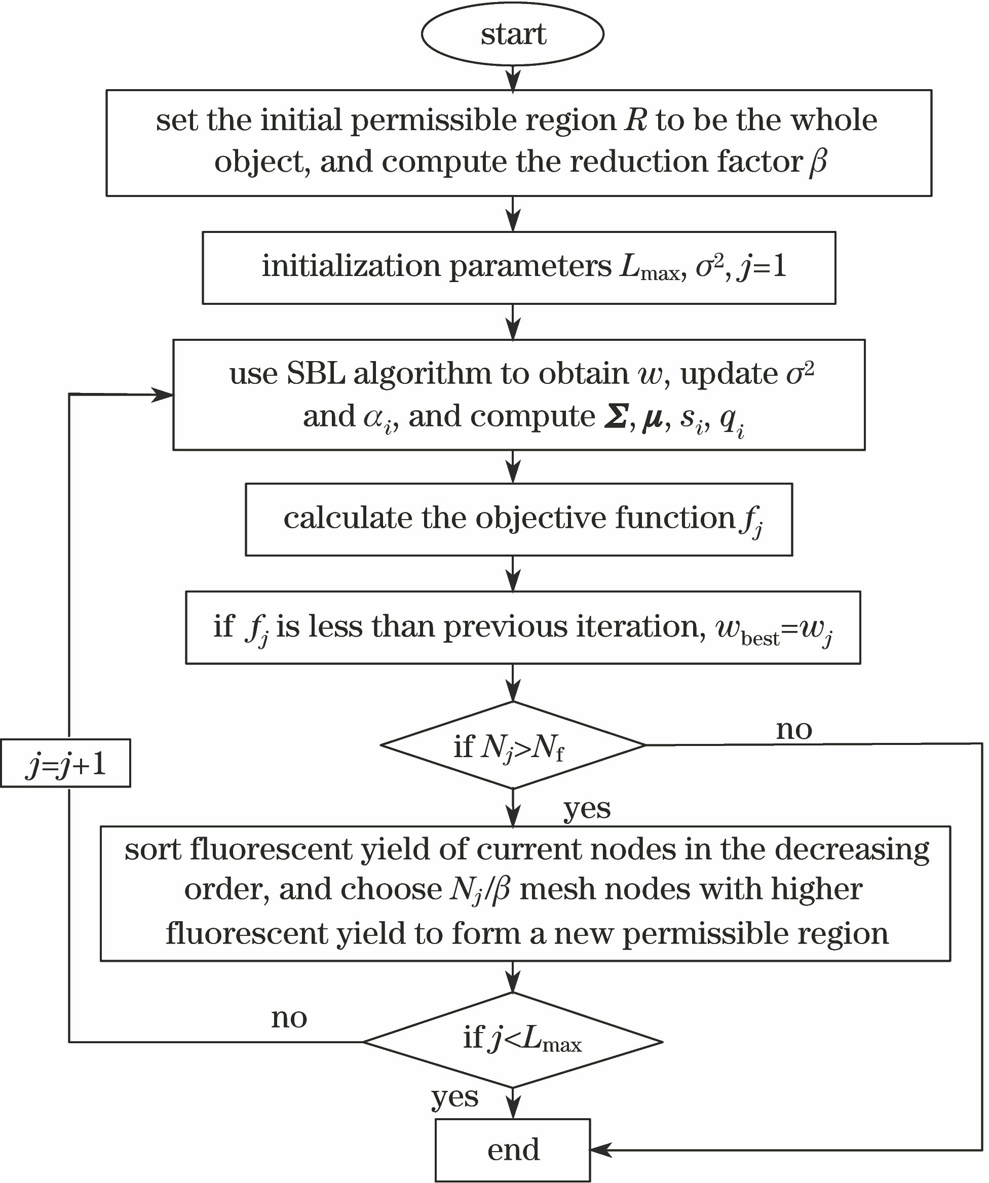
Fig. 1. SBL algorithm combined with iterative-shrinking permissible region strategy

Download full size

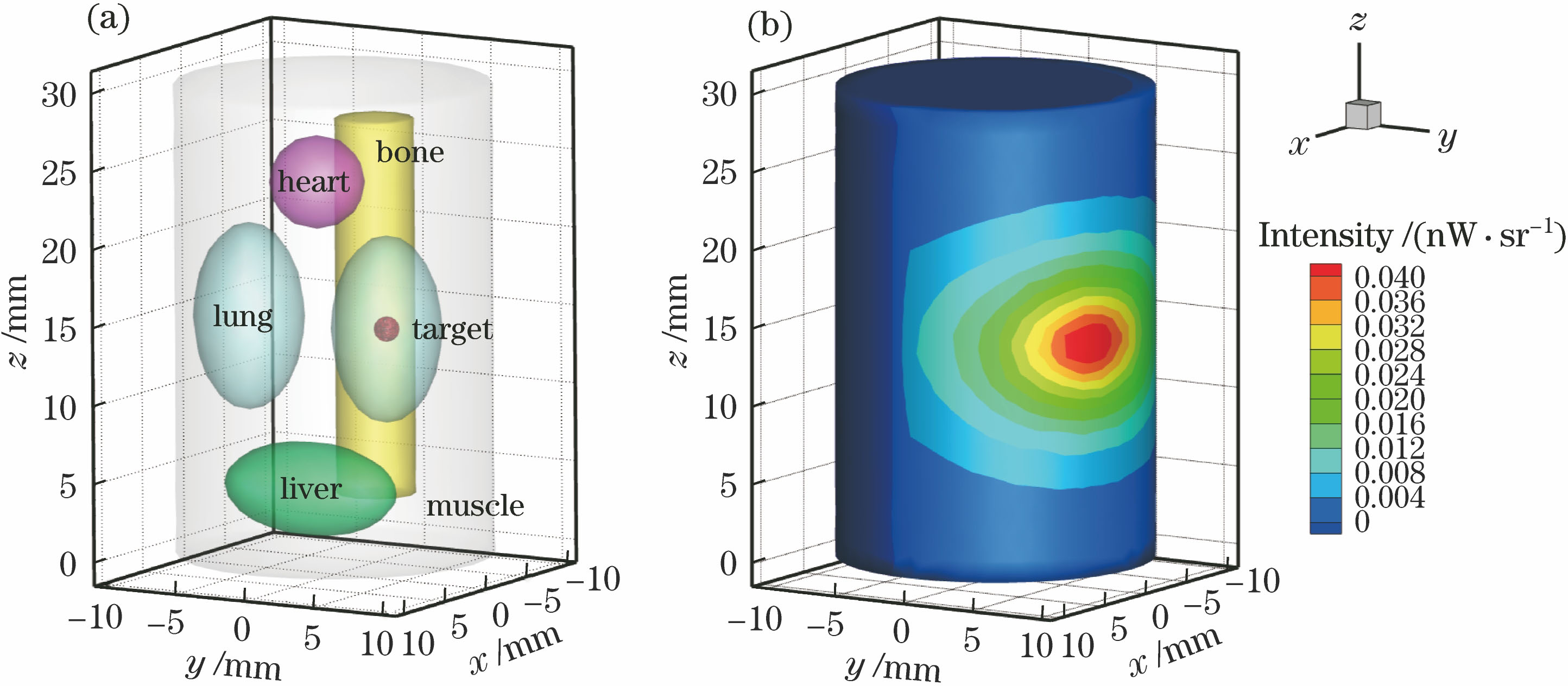
Fig. 2. (a) Model of non-homogeneous cylinder phantom; (b) surface optical information

Download full size

Fig. 3. Reconstruction results of simulation experiments. (a)-(c) Stereograms of reconstruction results with IVTCG, StOMP, and SBL; (d)-(f) two-dimensional cross-section views with the three algorithms at z=15 mm

Download full size

Fig. 4. Results of preliminary experiment 1. (a) Pseudocolor images collected by IVIS system (first column represents results of experimental group, while second column represents results of control group); (b) quantification analysis results of Fig. 4(a)

Download full size

Fig. 5. Results of preliminary experiment 2. (a) Pseudocolor images collected by IVIS system; (b) quantification analysis results of Fig. 5(a)

Download full size

Fig. 6. Geometric structure diagrams of (a) cubic and (b) cylindrical phantom; single-views of (c) cubic and (d) cylindrical phantoms collected by IVIS system

Download full size

Fig. 7. Reconstruction results of cubic physical phantom experiment. (a)-(c) Stereograms of reconstruction results with IVTCG, StOMP, and SBL; (d)-(f) two-dimensional cross-section views of three algorithms at z=1 mm

Download full size

Fig. 8. Reconstruction results of cylindrical physical phantom experiment. (a)-(c) Stereograms of reconstruction results with IVTCG, StOMP, and SBL; (d)-(f) two-dimensional cross-section views of three algorithms at z=1 mm

Download full size

Organ	$\begin{matrix} {μ_{a}}_{} \end{matrix}$ /mm^-1	$\begin{matrix} {μ_{s}}_{} \end{matrix}$ /mm^-1	g
Muscle	0.0052	10.800	0.90
Heart	0.0083	6.733	0.85
Lung	0.0133	19.700	0.90
Liver	0.0329	7.000	0.90
Bone	0.0060	60.090	0.90

Table 1. Optical parameters of different regions of non-homogeneous cylinder phantom

Algorithms	Actual source central position /mm	Reconstructed source central position /mm	$\begin{matrix} {f_{LE}}_{} \end{matrix}$ /mm	f_Dice	Time /s
IVTCG	(2,5,15)	(1.72,4.11,12.36)	2.81	0	1.38
StOMP	(2,5,15)	(2.66,5.92,15.54)	1.26	0.33	0.74
SBL	(2,5,15)	(2.09,5.35,15.51)	0.63	0.50	0.58

Table 2. Results of three reconstruction algorithms in simulation experiment

Noise level /%	Actual source central position /mm	Reconstructed source central position /mm	$\begin{matrix} {f_{LE}}_{} \end{matrix}$ /mm	f_Dice	Time /s
10	(2,5,15)	(2.08,5.38,15.51)	0.64	0.50	0.71
20	(2,5,15)	(2.07,5.40,15.52)	0.66	0.45	0.68
30	(2,5,15)	(2.19,5.57,14.60)	0.72	0.40	0.74
40	(2,5,15)	(2.38,5.36,15.51)	0.73	0.40	0.70

Table 3. Reconstruction results of SBL algorithms at different noise levels

Algorithm	Actual source central position /mm	Reconstructed source central position /mm	$\begin{matrix} {f_{LE}}_{} \end{matrix}$ /mm	f_Dice	Time /s
IVTCG	(6.25,0,1.00)	(5.23,0.73,-1.40)	2.71	0	4.45
StOMP	(6.25,0,1.00)	(5.54,1.48,0.71)	1.66	0.13	2.82
SBL	(6.25,0,1.00)	(6.08,-0.26,0.42)	0.66	0.50	1.97

Table 4. Results of three reconstruction algorithms in cubic physical phantom experiment

Algorithm	Actual source central position /mm	Reconstructed source central position /mm	$\begin{matrix} {f_{LE}}_{} \end{matrix}$ /mm	f_Dice	Time /s
IVTCG	(6.25,0,1.00)	(5.62,-0.22,-2.01)	3.08	0	4.72
StOMP	(6.25,0,1.00)	(5.19,-0.54,0.56)	1.27	0.29	2.98
SBL	(6.25,0,1.00)	(6.59,-0.07,0.47)	0.63	0.50	1.87

Table 5. Results of three reconstruction algorithms in cylindrical physical phantom experiment

Yuqing Hou, Hua Xue, Xin Cao, Haibo Zhang, Xuan Qu, Xiaowei He. Single-View Enhanced Cerenkov Luminescence Tomography Based on Sparse Bayesian Learning[J]. Acta Optica Sinica, 2017, 37(12): 1217001

Download Citation

Set citation alerts for the article

Tools

Set citation alerts for the article

Save the article for my favorites

Paper Information