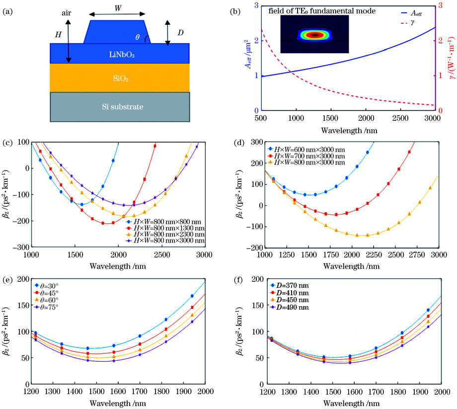
Fig. 1. LiNbO₃ waveguide structure and dispersion engineering of TE₀ fundamental mode. (a) LiNbO₃ waveguide structure; (b) A_eff and γ of TE₀ mode; (c) simulation on GVD versus W; (d) simulation on GVD versus H; (e) simulation on GVD versus θ; (f) simulation on GVD versus D

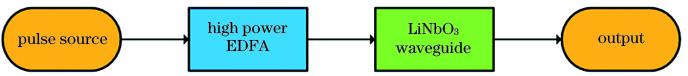
Fig. 2. Structural diagram of high repetition rate flat optical frequency comb generation

Fig. 3. Simulation results of initial chirp-free hyperbolic secant pulse propagating in nonlinear LiNbO₃ waveguide with normal dispersion. Evolution of pulse envelopes in (a1) time and (a2) frequency domains; pulse envelopes in (b1) time and (b2) frequency domains after pulse propagation of 3.6 m

Fig. 4. Evolution of periodic pulse propagating in nonlinear LiNbO₃ waveguide with normal dispersion.(a) Two-dimensional evolution process; (b) 3D evolution process

Fig. 5. Spectrograms of initial chirp-free hyperbolic secant pulse at various propagation distances. (a) 0; (b) 1.5 m;(c) 3.6 m; (d) 6.0 m

Fig. 6. Spectrograms of initial chirp-free Gaussian pulse at various propagation distances. (a) 0; (b) 1.2 m;(c) 2.0 m; (d) 4.2 m

Fig. 7. Spectrograms of initial chirp-free third-order super-Gaussian pulse at various propagation distances. (a) 0;(b) 0.6 m; (c) 1.2 m; (d) 2.4 m

Fig. 8. Final broadening spectra and pulse envelopes in time domain after propagation through 3.6 m long waveguide when only one parameter is changed and the other parameters are fixed. (a) Only β₂ changes; (b) only P₀ changes; (c) only T₀ changes; (d) only β₃ changes; (e) only C changes; (f) only α changes; (g) only input pulse envelope changes

Fig. 9. Coherence of optical frequency comb generated by hyperbolic secant pulse propagating in 3.6 m long LiNbO₃ waveguide

Table 1. Parameters used in simulation