The past two decades or so have witnessed the rapid development of laser wakefield acceleration (LWFA) since the experimentally obtained mono-energetic electron beam^[1^–3^]. From the early stage of tens of percent level energy spread and few mm mrad-level emittance, LWFA electron beams have now achieved electron beams with nC-level charge^[4^,5^], few per-mille-level relative energy spread^[6^–9^] and sub-mm mrad-level emittance^[10^]. Benefitted from the ultra-high acceleration gradient of LWFA^[11^–15^], ultra-compact radiation sources, such as betatron radiation^[16^–18^], Compton scattering^[19^–22^] and tabletop free electron lasers (FELs)^[23^–25^], injectors for future colliders^[26^] will be possible. Most LWFA-based applications require an excellent 6D electron beam brightness^[27^,28^], defined by ${B}_{6\mathrm{D}} = \frac{I_{\mathrm{P}}}{\varepsilon_{nx}{\varepsilon}_{ny}{\sigma}_{\gamma}\cdot 0.1\%}$ , where ${I}_{\mathrm{P}}$ is the peak current, ${\sigma}_{\gamma}$ is the relative energy spread and ${\varepsilon}_{nx}$ and ${\varepsilon}_{ny}$ are the normalized transverse emittance of the electron beam. As a critical parameter, the transverse emittance needs to be accurately diagnosed.

Owing to the large instability in the plasma acceleration process, a single-shot high-resolution diagnostic method is preferable. At present, one of commonly used single-shot emittance measurement methods is the ‘pepper-pot’ method^[29^]. It uses a beam-intercepting mask to construct the electron beam phase space distribution through the divergence and charge of electrons passing through the hole, in which it is preferrable to have a beam with a large charge (higher than tens of pC level). Ref. [30] reports that this method is not suitable for LWFA beams owing to large divergence. The radiation-based method^[31^–33^] measures the transverse size of the electron beam inside the bubble and the divergence outside the bubble. Neglecting the evolution as the electron beam leaves the bubble will make the measured result deviate from its true emittance^[34^]. In comparison, the direct energy-dispersed measurement method using a focused beam transfer line and an energy spectrometer has greater feasibility, and is suitable for low-charge electron beam diagnostics^[10^,35^]. Unlike the early quadrupole scanning method^[36^], the electron beam has energy-dependent transverse deflection through the dipole, which separates the influence of chromaticity effects^[37^] while measuring sizes. This method can not only measure the emittance, but also obtain the transverse phase space distribution of the electron beam.

In this paper, a single-shot method for measuring the energy-sliced emittance of the electron beam was demonstrated experimentally. Through analyzing the evolution of the electron transverse trajectory in the bubble, the phase difference of the electrons with respect to the central energy can be estimated. Phase compensation unifies the electron beam phase, which makes the phase space present the slice information of the electron beam. The slice emittance is then calculated by fitting to the vertical sizes of the electron beam sliced at different energies. In order to more accurately reflect the whole process of the electron beam from its inception to final measurement, Fourier–Bessel particle-in-cell (FBPIC) simulation was also carried out. The simulation results are in good agreement with the experimental results, indicating the accuracy of the analysis.

While accelerated in the nonlinear plasma wake (the so-called bubble), the electrons experience transverse oscillation^[38^], which causes the evolution of the beam emittance. Considering a relativistic electron accelerates and oscillates in the bubble, the transverse trajectory can be expressed as $r = {R}_{\mathrm{r}}\cdot \cos \left({k}_{\beta}z- ct\right)$ in a linear focus field. It is thereby obtained that an electron with energy $\gamma$ rotates with a frequency of ${\omega}_{\beta} = c{k}_{\beta} = c{k}_{\mathrm{p}}/\sqrt{2\gamma }$ in the phase space $\left(r,{p}_{\mathrm{r}}\right)$ , where ${k}_{\beta}$ is the betatron oscillation wave number and ${k}_{\mathrm{p}}$ is the plasma wave number. 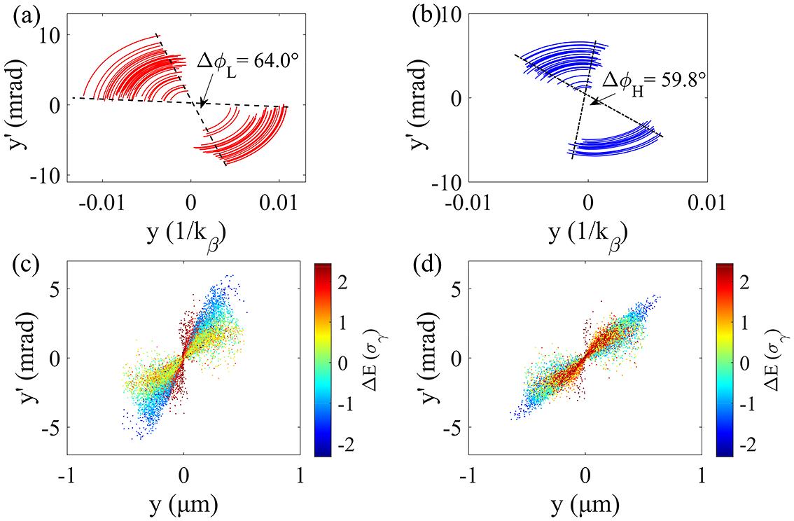Figures 1(a) and 1(b) show the phase space trajectories of the low-energy part and the high-energy part in one electron beam within the same duration. The energy-dependent rotational frequency of electrons in the phase space results in different phase advances ( ${\Delta {\phi}_{\mathrm{H}}\ne \Delta {\phi}_{\mathrm{L}}}$ ). According to Refs. [39,40], the phase advance of the electron can be obtained by the integral formula $\phi = \int \mathrm{d}t{\omega}_{\beta}$ . The energy gain per unit length can be regarded as a constant ${\gamma}^{\prime} = e{E}_{\mathrm{z}}/m{c}^2$ in the case of ignoring the phase slippage. Therefore, the electron phase advance can be denoted as follows:

$$\begin{align}\phi = \frac{\sqrt{2}{k}_{\mathrm{p}}}{\gamma^{\prime }}\left(\sqrt{\gamma (0)+{\gamma}^{\prime }l}-\sqrt{\gamma (0)}\right),\end{align}$$  (1)

where $\gamma (0)$ and $\gamma (l) = \gamma (0)+{\gamma}^{\prime }l$ represents the initial energy and the energy of the electron after acceleration length l, respectively. Considering the initial phase difference $\Delta {\phi}_0$ in the injection stage, the phase difference of the electrons can be expressed as follows:

$$\begin{align}\Delta \phi (l) = {\phi}_{\mathrm{H}}(l)-{\phi}_{\mathrm{L}}(l)+\Delta {\phi}_0,\end{align}$$  (2)

where ${\phi}_{\mathrm{H}}(l)$ and ${\phi}_{\mathrm{L}}(l)$ following Equation (1) represent the phase advance of high-energy and low-energy electrons, respectively. Therefore, the phase difference of the electrons owing to the energy spread in bubble is inevitable. Through the electron beam transverse oscillation analysis^[41^], different energy slices can be phase compensated to the same phase by matrix $N\left(\Delta \phi \right)$ .

In the framework of beam optics, the single-electron state can be characterized by a 6D vector. In the case of ignoring the second-order effect, the trajectory of the single electron through the transfer line can be expressed as follows:

$$\begin{align}\left(\begin{array}{@{}c@{}}r\\ {}{r}^{\prime}\end{array}\right) {=} \left(\begin{array}{@{}cc@{}}{M}_{11}& {M}_{12}\\ {}{M}_{21}& {M}_{22}\end{array}\right)\!\left(\begin{array}{@{}c@{\ }c@{}}\cos \left(\Delta \phi \right)& \sin \left(\Delta \phi \right)/{k}_{\beta}\\ {}-{k}_{\beta}\cdot \sin \left(\Delta \phi \right)& \cos \left(\Delta \phi \right)\end{array}\right)\!\left(\begin{array}{@{}c@{}}{r}_0\\ {}{r}_0^{\prime}\end{array}\right)\!,\end{align}$$  (3)

where $r$ and ${r}^{\prime }$ represent the transverse position (horizontal or vertical) and divergence of the electron at the end of the beamline, respectively and ${r}_0$ and ${r}_0^{\prime }$ represent the transverse position (horizontal or vertical) and divergence of the electron with phase compensation at the beginning of the beamline, respectively. The first term on the right-hand side of the equation represents the beamline transfer matrix M, and the second term $N\left(\Delta \phi \right)$ is the phase compensation term for the electron relative to the reference one with central energy. Figure 1(c) shows the transverse energy-dependent phase space distribution of the electron beam. When the phase is compensated with respect to the central energy, as shown in Figure 1(d), electrons with different energies have the same phase and the slice emittance diagnosis can be feasible. The vertical size of the beam at the end of the beamline can be represented by the statistic ${\sigma}_y^2 = \left\langle {\left(y-{y}_{\mathrm{c}}\right)}^2\right\rangle$ , where ${y}_{\mathrm{c}}$ is the vertical center position of the electron beam, which generally defaults to zero considering that the electron beam transports along the main optical axis. According to Equation (3) and the above equation, the vertical size of the electron beam can be expressed by the transfer matrix and the initial parameters of the electron beam as follows^[42^]:

$$\begin{align}{\sigma}_y^2 = {R}_{11}^2\varepsilon {\beta}_0-2{R}_{11}{R}_{12}\varepsilon {\alpha}_0+{R}_{12}^2\varepsilon {\gamma}_0,\end{align}$$  (4)

where ${\alpha}_0$ , ${\beta}_0$ and ${\gamma}_0$ are the initial Twiss parameters of the electron beam in the vertical direction and satisfy the equation ${\alpha}_0^2+1 = {\beta}_0\cdot {\gamma}_0$ and ${R}_{11}$ and ${R}_{12}$ represent the elements in the total matrix $R = M\cdot N\left(\Delta \phi \right)$ with the phase compensated. It is noted that the transfer matrix elements of the quadrupoles are correlated with its focus strength $K = eB/\gamma mac$ , where e and m are the charge and mass of the electron, respectively, $B/a$ represents the magnetic field gradient, γ is the Lorentz factor and c is the speed of light in vacuum. For a given beamline, the transfer matrix is determined only by the electron energy, which means that the vertical size of the electron beam at the end of the beam line is related to the electron beam energy. The vertical size of the electron beam at the focal point is the smallest and increases with the energy shift. The initial transverse slice emittance can be determined by the direct measurement of such energy-resolved beam size.

Figure 2(a) shows a schematic diagram of the experimental setup for the emittance diagnostic of high-quality electron beams produced by the LWFA. The experiments were performed on a Ti:sapphire chirped pulse amplification laser system with 30-fs pulse duration, 200-TW peak power and 1 Hz repetition rate at the Shanghai Institute of Optics and Fine Mechanics (SIOM)^[43^]. An 800-nm laser pulse with an on-target power of approximately 120 TW was focused onto a gas target by an f/30 off-axis parabolic mirror, and the vacuum beam radius ω₀ was measured to be 32 μm full width at half maximum (FWHM). The fractional laser energy contained in the laser spot was measured to be approximately 61% at 1/e², and the peak intensity was estimated to be 4.3 × 10¹⁸ W/cm², corresponding to a normalized amplitude of a₀ ≈ 1.3.

The pure helium gas was sprayed from a supersonic gas nozzle to the metal target to conduct a structured gas flow with a shock front. The longitudinal density profile can be adjusted by varying the relative position between the nozzle and the target and the gas back pressure. A Michelson-type interferometer with a 4-f optical imaging system was used for measuring the plasma density, as shown in Figure 2(b). The shock front has a peak density of (4 ± 0.5) × 10¹⁸ cm^–3, following which is a 3-mm-long plateau with the density of (2.2 ± 0.4) × 10¹⁸ cm^–3. The beamline is composed of three quadrupole magnets, where the first two are permanent quadrupoles with a magnetic field gradient of 250 T/m, and the third one is an electromagnetic quadrupole whose magnetic field gradient is tunable in the range of 0–80 T/m. The accelerated electron beam is deflected onto a Lanex phosphor screen (Y₃Al₅O₁₂:Ce³⁺) by a 90-cm-long tunable dipole magnet. The energy spectrometer has an energy resolution of 0.011% at 500 MeV. The total beamline has a length of approximately 2.4 m from the gas target to the electron spectrometer, and the components in the beamline were aligned within ±100 μm of coaxiality with the main optical axis.

It is noted that only the linear beam optics are applied in the aforementioned theoretical model for simplification. The transport effects up to the second order and the space charge are considered in the simulation. By adjusting the relative position between the two permanent magnetic quadrupoles and the magnetic field gradient of the electromagnetic quadrupole, the focused beamline was optimized with a cancelling term ${M}_{12}$ for the central energy electrons (~500 MeV) to a waist^[10^,35^]. The element ${M}_{11}$ in the transfer matrix then represents the magnification of the transverse beam size, which is estimated to be –11 in the presented beamline and is sufficient for the high-precision measurement of the energy-resolved sizes. Under optimized conditions, Figure 2(d) shows a typical electron beam energy spectrum with a center energy of around 500 MeV, a relative energy spread of 0.5% and an average charge of about 30 pC. The energy fluctuation of the electron beam measured by 10 consecutive shots is less than 3%.

Figure 3(a) shows a typical energy spectrum of the focused electron beam deflected by the dipole, with the intensity corresponding to the relative charge density. The root-mean-square (RMS) energy-resolved beam size can be obtained by weighted counting of the distance of the electrons from the beam center in the vertical direction. Intensities lower than 10% of the peak intensities in each energy slice are set to zero to avoid overestimation of the sizes. The blue line in Figure 3(b) represents the vertical size corresponding to different energy slices in Figure 3(a), and the red line is the fitting curve. Quasi-3D particle-in-cell simulations were performed using the FBPIC code^[44^–46^] to estimate the initial phase difference after injection, which cannot be directly measured in the experiment. The simulation parameters were chosen according to the experiments. The initial phase difference was estimated to be 34.2° after injection, as shown in Figure 3(c), where the horizontal axis represents the final relative energy of the tracking electrons. The range from ${E}_{\mathrm{c}}-2{\sigma}_{\gamma}$ to ${E}_{\mathrm{c}}+2{\sigma}_{\gamma}$ was used in the estimation of the phase difference, where ${E}_{\mathrm{c}}$ and ${\sigma}_{\gamma}$ represent the center energy and RMS energy spread, respectively. The maximum phase difference between each slice of the electron beam is approximately 107° (blue solid line), which is very close to the calculated value of 105.6° (pink dotted line) according to Equation (2). The small deviation between the simulation and the calculation is mainly caused by the non-constant acceleration field. The normalized energy-sliced emittance of the electron beam can then be calculated to be approximately 0.27 mm mrad after the compensation of the total phase difference. Ref. [24] shows the full FBPIC simulation results with vertical slice emittances ranging from 0.18 to 0.48 mm mrad. The simulation shows that the electron beam average slice emittance is approximately 0.26 mm mrad in the vertical direction, which is in good agreement with the experiments and analysis.

Figure 4 shows the measured normalized emittance for various beam charges with the back pressures of 1.5 and 2 bar, respectively. Each data point represents 20 consecutive shots. The electron beam emittance is lower at the back pressure of 1.5 bar and fluctuates in the range of 0.27–0.34 mm mrad. Most of the emittance fluctuates in the range of 0.28–0.36 mm mrad, and the highest value can reach approximately 0.45 mm mrad under the condition of 2 bar back pressure. In general, the energy-sliced emittance shows no significant correlation with the beam charge. Compared with the back pressure of 2 bar, the electron beam emittance fluctuation is smaller when the back pressure is 1.5 bar. In particular, when the charge amount is higher than 20 pC, the electron beam emittance fluctuates greatly.

The assumption that the electron beam transports along the main optical axis is made in the aforementioned theoretical model. However, positional deviation occurs due to the shot-to-shot pointing fluctuations of the electron beam from the LWFAs. An initial pointing deviation of P will result in a positional offset ${M}_{12}\cdot P$ at the end of the beamline. Figure 5(a) shows a typical electron beam imaging on a phosphor screen with an initial vertical pointing deviation. The position of the electrons at the beam waist does not shift due to the zero transfer term ${M}_{12}$ at the focal point. Near the focal point, the transfer term ${M}_{12}$ is approximately linear with the energy, which is in good agreement with the measured result.

The red dashed line in Figure 5(a) is a slice perpendicular to the electron beam distribution, and the white dashed line is a slice with the same horizontal offset relative to the main optical axis. The red and the blue curves in Figure 5(b) indicate the RMS energy-resolved beam size by weighted counting of the distance of the electrons from the beam center along the dashed red and white lines in Figure 5(a). Although the design ensures that the horizontal focal point locates at the end of the beamline, the coupling of the horizontal position deviation and the deflection angle in the dipole means that any slice on the screen with the same horizontal offset is not absolutely mono-energetic. The measured sizes increase as electron beams with different energies generate additional vertical offset, owing to pointing jitter. Figure 5(c) shows the relative charge distributions of the two profiles corresponding to Figure 5(a), in which the subgraphs are locally enlarged graphs. The dashed line represents the Gaussian fitting profiled by the red line, with a fitting threshold of 50% of the peak value. It can be seen from the Figure 5(c) that the electron beam is approximately Gaussian in the vertical direction. The greater weight of the background noise in the low-intensity signal and the transverse divergence of the electron beam owing to space charge effects make the beam profile slightly larger than the Gaussian curve. Figure 2(c) shows the center position of 62 consecutive electron beams, and the vertical RMS pointing jitter of the electron beam is 0.52 mrad (the pointing fluctuation was measured by a beam position monitor located 4 m from the gas target, where the quadrupoles were turned off). Considering the effect of the pointing jitter within the double-RMS range, the red and blue lines in Figure 5(d) represent the imaging beam slope and the measured relative emittance derivation for different pointing jitters, respectively.

We experimentally performed single-shot measurements of electron beam slice emittance using a focused transfer line. The electron beam significantly follows envelope oscillations in the bubble owing to the linear focusing field. The coupling of the longitudinal acceleration field and the transverse focusing field results in an energy-dependent electron beam phase. Each slice phase is unified by means of phase compensation based on the relationship between the electron phase and energy. The emittance can be obtained through fitting the energy-dependent size calculated by weighted statistics. Electron beams with an average slice emittance as low as 0.27 mm mrad are currently experimentally available. Based on the transfer matrix, the pointing jitter can be obtained from the energy-dependent electron beam centroid offset, and the corresponding emittance derivation can also be measured. The simulation results based on the experimental parameters are in good agreement with the actual measurement results.

References

[1] J. Faure, Y. Glinec, A. Pukhov, S. Kiselev, S. Gordienko, E. Lefebvre, J. P. Rousseau, F. Burgy, V. Malka. Nature, 431, 541(2004).
[2] C. G. R. Geddes, C. Toth, J. van Tilborg, E. Esarey, C. B. Schroeder, D. Bruhwiler, C. Nieter, J. Cary, W. P. Leemans. Nature, 431, 538(2004).
[3] S. P. D. Mangles, C. D. Murphy, Z. Najmudin, A. G. R. Thomas, J. L. Collier, A. E. Dangor, E. J. Divall, P. S. Foster, J. G. Gallacher, C. J. Hooker, D. A. Jaroszynski, A. J. Langley, W. B. Mori, P. A. Norreys, F. S. Tsung, R. Viskup, B. R. Walton, K. Krushelnick. Nature, 431, 535(2004).
[4] J. P. Couperus, R. Pausch, A. Kohler, O. Zarini, J. M. Kramer, M. Garten, A. Huebl, R. Gebhardt, U. Helbig, S. Bock, K. Zeil, A. Debus, M. Bussmann, U. Schramm, A. Irman. Nat. Commun., 8(2017).
[5] J. Gotzfried, A. Dopp, M. F. Gilljohann, F. M. Foerster, H. Ding, S. Schindler, G. Schilling, A. Buck, L. Veisz, S. Karsch. Phys. Rev. X, 10, 041015(2020).
[6] L. T. Ke, K. Feng, W. T. Wang, Z. Y. Qin, C. H. Yu, Y. Wu, Y. Chen, R. Qi, Z. J. Zhang, Y. Xu, X. J. Yang, Y. X. Leng, J. S. Liu, R. X. Li, Z. Z. Xu. Phys. Rev. Lett., 126, 214801(2021).
[7] Y. P. Wu, J. F. Hua, Z. Zhou, J. Zhang, S. Liu, B. Peng, Y. Fang, Z. Nie, X. N. Ning, C. H. Pai, Y. C. Du, W. Lu, C. J. Zhang, W. B. Mori, C. Joshi. Phys. Rev. Lett., 122, 204804(2019).
[8] R. D’Arcy, S. Wesch, A. Aschikhin, S. Bohlen, C. Behrens, M. J. Garland, L. Goldberg, P. Gonzalez, A. Knetsch, V. Libov, A. M. de la Ossa, M. Meisel, T. J. Mehrling, P. Niknejadi, K. Poder, J. H. Rockemann, L. Schaper, B. Schmidt, S. Schroder, C. Palmer, J. P. Schwinkendorf, B. Sheeran, M. J. V. Streeter, G. Tauscher, V. Wacker, J. Osterhoff. Phys. Rev. Lett., 122, 034801(2019).
[9] V. Shpakov, M. P. Anania, M. Bellaveglia, A. Biagioni, F. Bisesto, F. Cardelli, M. Cesarini, E. Chiadroni, A. Cianchi, G. Costa, M. Croia, A. Del Dotto, D. Di Giovenale, M. Diomede, M. Ferrario, F. Filippi, A. Giribono, V. Lollo, M. Marongiu, V. Martinelli, A. Mostacci, L. Piersanti, G. Di Pirro, R. Pompili, S. Romeo, J. Scifo, C. Vaccarezza, F. Villa, A. Zigler. Phys. Rev. Lett., 122, 114801(2019).
[10] S. K. Barber, J. van Tilborg, C. B. Schroeder, R. Lehe, H. E. Tsai, K. K. Swanson, S. Steinke, K. Nakamura, C. G. R. Geddes, C. Benedetti, E. Esarey, W. P. Leemans. Phys. Rev. Lett., 119, 104801(2017).
[11] W. P. Leemans, B. Nagler, A. J. Gonsalves, C. Toth, K. Nakamura, C. G. R. Geddes, E. Esarey, C. B. Schroeder, S. M. Hooker. Nat. Phys., 2, 696(2006).
[12] W. P. Leemans, A. J. Gonsalves, H. S. Mao, K. Nakamura, C. Benedetti, C. B. Schroeder, C. Toth, J. Daniels, D. E. Mittelberger, S. S. Bulanov, J. L. Vay, C. G. R. Geddes, E. Esarey. Phys. Rev. Lett., 113, 245002(2014).
[13] A. J. Gonsalves, K. Nakamura, J. Daniels, C. Benedetti, C. Pieronek, T. C. H. de Raadt, S. Steinke, J. H. Bin, S. S. Bulanov, J. van Tilborg, C. G. R. Geddes, C. B. Schroeder, C. Toth, E. Esarey, K. Swanson, L. Fan-Chiang, G. Bagdasarov, N. Bobrova, V. Gasilov, G. Korn, P. Sasorov, W. P. Leemans. Phys. Rev. Lett., 122, 084801(2019).
[14] X. M. Wang, R. Zgadzaj, N. Fazel, Z. Y. Li, S. A. Yi, X. Zhang, W. Henderson, Y. Y. Chang, R. Korzekwa, H. E. Tsai, C. H. Pai, H. Quevedo, G. Dyer, E. Gaul, M. Martinez, A. C. Bernstein, T. Borger, M. Spinks, M. Donovan, V. Khudik, G. Shvets, T. Ditmire, M. C. Downer. Nat. Commun., 4(2013).
[15] M. Turner, A. J. Gonsalves, S. S. Bulanov, C. Benedetti, N. A. Bobrova, V. A. Gasilov, P. V. Sasorov, G. Korn, K. Nakamura, J. van Tilborg, C. G. Geddes, C. B. Schroeder, E. Esarey. High Power Laser Sci. Eng., 9, e17(2021).
[16] J. B. Svensson, D. Guenot, J. Ferri, H. Ekerfelt, I. G. Gonzalez, A. Persson, K. Svendsen, L. Veisz, O. Lundh. Nat. Phys., 17, 639(2021).
[17] M. Kozlova, I. Andriyash, J. Gautier, S. Sebban, S. Smartsev, N. Jourdain, U. Chulagain, Y. Azamoum, A. Tafzi, J. P. Goddet, K. Oubrerie, C. Thaury, A. Rousse, K. T. Phuoc. Phys. Rev. X, 10, 011061(2020).
[18] J. C. Wood, D. J. Chapman, K. Poder, N. C. Lopes, M. E. Rutherford, T. G. Whites, F. Albert, K. T. Behm, N. Booth, J. S. J. Bryant, P. S. Foster, S. Glanzer, E. Hill, K. Krushelnick, Z. Najmudin, B. B. Pollock, S. Rose, W. Schumaker, R. H. H. Scott, M. Sherlock, A. G. R. Thomas, Z. Zhao, D. E. Eakins, S. P. D. Mangles. Sci. Rep., 8(2018).
[19] S. Chen, N. D. Powers, I. Ghebregziabher, C. M. Maharjan, C. Liu, G. Golovin, S. Banerjee, J. Zhang, N. Cunningham, A. Moorti, S. Clarke, S. Pozzi, D. P. Umstadter. Phys. Rev. Lett., 110, 155003(2013).
[20] K. Khrennikov, J. Wenz, A. Buck, J. Xu, M. Heigoldt, L. Veisz, S. Karsch. Phys. Rev. Lett., 114, 195003(2015).
[21] K. T. Phuoc, S. Corde, C. Thaury, V. Malka, A. Tafzi, J. P. Goddet, R. C. Shah, S. Sebban, A. Rousse. Nat. Photonics, 6, 308(2012).
[22] J. M. Cole, K. T. Behm, E. Gerstmayr, T. G. Blackburn, J. C. Wood, C. D. Baird, M. J. Duff, C. Harvey, A. Ilderton, A. S. Joglekar, K. Krushelnick, S. Kuschel, M. Marklund, P. McKenna, C. D. Murphy, K. Poder, C. P. Ridgers, G. M. Samarin, G. Sarri, D. R. Symes, A. G. R. Thomas, J. Warwick, M. Zepf, Z. Najmudin, S. P. D. Mangles. Phys. Rev. X, 8, 011020(2018).
[23] K. Nalkajima. Nat. Phys., 4, 92(2008).
[24] W. T. Wang, K. Feng, L. T. Ke, C. H. Yu, Y. Xu, R. Qi, Y. Chen, Z. Y. Qin, Z. J. Zhang, M. Fang, J. Q. Liu, K. N. Jiang, H. Wang, C. Wang, X. J. Yang, F. X. Wu, Y. X. Leng, J. S. Liu, R. X. Li, Z. Z. Xu. Nature, 595, 516(2021).
[25] C. Emma, J. Van Tilborg, R. Assmann, S. Barber, A. Cianchi, S. Corde, M. E. Couprie, R. D’Arcy, M. Ferrario, A. F. Habib, B. Hidding, M. J. Hogan, C. B. Schroeder, A. Marinelli, M. Labat, R. Li, J. Liu, A. Loulergue, J. Osterhoff, A. R. Maier, B. W. J. McNeil, W. Wang. High Power Laser Sci. Eng., 9, e57(2021).
[26] K. Nakajima, J. Wheeler, G. Mourou, T. Tajima. Int. J. Mod. Phys. A, 34, 1943003(2019).
[27] G. G. Manahan, A. F. Habib, P. Scherkl, P. Delinikolas, A. Beaton, A. Knetsch, O. Karger, G. Wittig, T. Heinemann, Z. M. Sheng, J. R. Cary, D. L. Bruhwiler, J. B. Rosenzweig, B. Hidding. Nat. Commun., 8, 15705(2017).
[28] S. Di Mitri, M. Cornacchia. Phys. Rept. Lett., 539(2014).
[29] C. M. S. Sears, A. Buck, K. Schmid, J. Mikhailova, F. Krausz, L. Veisz. Phys. Rev. Spec. Top. Accel. Beams, 13, 092803(2010).
[30] A. Cianchi, M. P. Anania, M. Bellaveglia, M. Castellano, E. Chiadroni, M. Ferrario, G. Gatti, B. Marchetti, A. Mostacci, R. Pompili, C. Ronsivalle, A. R. Rossi, L. Serafini. Nucl. Instrum. Methods Phys. Res. Sect. A, 720, 153(2013).
[31] G. R. Plateau, C. G. R. Geddes, D. B. Thorn, M. Chen, C. Benedetti, E. Esarey, A. J. Gonsalves, N. H. Matlis, K. Nakamura, C. B. Schroeder, S. Shiraishi, T. Sokollik, J. van Tilborg, C. Toth, S. Trotsenko, T. S. Kim, M. Battaglia, T. Stohlker, W. P. Leemans. Phys. Rev. Lett., 109, 064802(2012).
[32] M. Schnell, A. Savert, B. Landgraf, M. Reuter, M. Nicolai, O. Jackel, C. Peth, T. Thiele, O. Jansen, A. Pukhov, O. Willi, M. C. Kaluza, C. Spielmann. Phys. Rev. Lett., 108, 075001(2012).
[33] C. Emma, A. Edelen, M. J. Hogan, B. O’Shea, G. White, V. Yakimenko. Phys. Rev. Accel. Beams, 21, 112802(2018).
[34] M. C. Downer, R. Zgadzaj, A. Debus, U. Schramm, M. C. Kaluza. Rev. Mod. Phys., 90, 035002(2018).
[35] S. K. Barber, J. H. Bin, A. J. Gonsalves, F. Isono, J. van Tilborg, S. Steinke, K. Nakamura, A. Zingale, N. A. Czapla, D. Schumacher, C. B. Schroeder, C. G. R. Geddes, W. P. Leemans, E. Esarey. Appl. Phys. Lett., 116, 234108(2020).
[36] R. Weingartner, S. Raith, A. Popp, S. Chou, J. Wenz, K. Khrennikov, M. Heigoldt, A. R. Maier, N. Kajumba, M. Fuchs, B. Zeitler, F. Krausz, S. Karsch, F. Gruner. Phys. Rev. Spec. Top. Accel. Beams, 15, 111302(2012).
[37] J. van Tilborg, S. Steinke, C. G. R. Geddes, N. H. Matlis, B. H. Shaw, A. J. Gonsalves, J. V. Huijts, K. Nakamura, J. Daniels, C. B. Schroeder, C. Benedetti, E. Esarey, S. S. Bulanov, N. A. Bobrova, P. V. Sasorov, W. P. Leemans. Phys. Rev. Lett., 115, 184802(2015).
[38] J. Feng, Y. F. Li, J. G. Wang, D. Z. Li, C. Q. Zhu, J. H. Tan, X. T. Geng, F. Liu, L. M. Chen. High Power Laser Sci. Eng., 9, e5(2021).
[39] X. L. Xu, J. F. Hua, F. Li, C. J. Zhang, L. X. Yan, Y. C. Du, W. H. Huang, H. B. Chen, C. X. Tang, W. Lu, P. Yu, W. An, C. Joshi, W. B. Mori. Phys. Rev. Lett., 112, 035003(2014).
[40] A. Koehler, R. Pausch, M. Bussmann, J. P. C. Cabadag, A. Debus, J. M. Kramer, S. Schobel, O. Zarini, U. Schramm, A. Irman. Phys. Rev. Accel. Beams, 24, 091302(2021).
[41] S. Corde, K. T. Phuoc, G. Lambert, R. Fitour, V. Malka, A. Rousse, A. Beck, E. Lefebvre. Rev. Mod. Phys., 85(2013).
[42] M. B. Reid. J. Appl. Phys., 70, 7185(1991).
[43] F. X. Wu, Z. X. Zhang, X. J. Yang, J. B. Hu, P. H. Ji, J. Y. Gui, C. Wang, J. C. Chen, Y. J. Peng, X. Y. Liu, Y. Q. Liu, X. M. Lu, Y. Xu, Y. X. Leng, R. X. Li, Z. Z. Xu. Opt. Laser Technol., 131, 106453(2020).
[44] M. Kirchen, R. Lehe, S. Jalas, O. Shapoval, J. L. Vay, A. R. Maier. Phys. Rev. E, 102, 013202(2020).
[45] S. Jalas, I. Dornmair, R. Lehe, H. Vincenti, J. L. Vay, M. Kirchen, A. R. Maier. Phys. Plasmas, 24, 033115(2017).
[46] R. Lehe, M. Kirchen, I. A. Andriyash, B. B. Godfrey, J. L. Vay. Comput. Phys. Commun., 203, 66(2016).
Set citation alerts for the article
Please enter your email address
© Copyright 2018-2021 | Chinese Laser Press. All Rights Reserved 沪ICP备15018463号-20