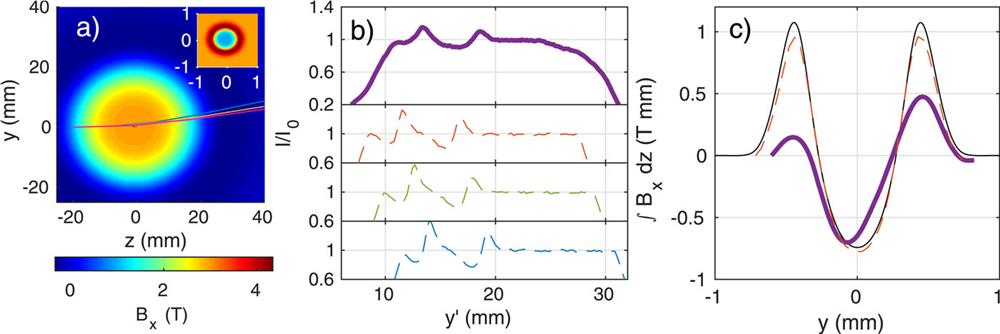
Fig. 1. (a) Example of the magnetic field structure, with a large background field surrounding a millimeter-scale signal region near the center (a close-up of which is shown in the inset on the top right). Overlaid are the paths of monoenergetic proton beams of energies 10 MeV (blue), 16 MeV (yellow), and 21 MeV (pink). (b) Example of three synthetic monoenergetic radiographs (dashed lines) at 10 MeV (blue), 12 MeV (green), and 14 MeV (red), compared with a composite combined radiograph (solid purple), modeled using a thermal proton distribution absorbed by a layer of RCF. (c) Magnetic field profile reconstructed from the combined blurred radiograph (bold purple line) compared with the true field profile (solid black) and the reconstruction from the monoenergetic radiograph at 14 MeV (dashed red).

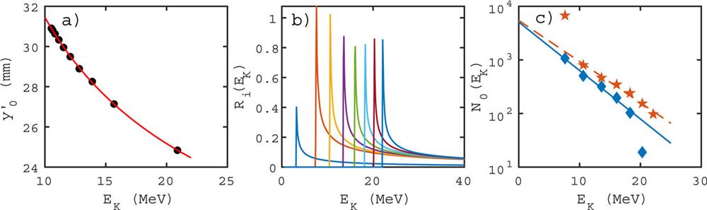
Fig. 2. (a) Deflection of the proton beam vs energy, measured by tracking the edge of the proton distribution in synthetic radiographs, and fitted to y0′(E)=a+b/E. (b) RCF absorption curves calculated by the finite element opacity model described in the text, with the first layer of RCF on the left. (c) Examples of proton energy distributions estimated from RCF doses measured on two different experimental laser shots, fitted to thermal distributions.

Fig. 3. (a) Examples of convolution kernels calculated for different RCF layers for a T = 5 MeV thermal proton spectrum (solid lines) passing through a 3 T background field, compared with the kernels for a T = 10 MeV proton spectrum under the same conditions (dotted lines). (b) Standard deviation of the kernels plotted vs the mean proton energy absorbed by each RCF layer, comparing T = 5 MeV and T = 10 MeV proton beams passing through a 3 T background field with a T = 5 MeV proton beam passing through a 10 T background field.

Fig. 4. (a) Synthetic radiographs from a thermal proton beam passing through a background field with a strength of 90 T mm before being absorbed by a layer of RCF. The combined radiograph (purple line) and that after application of deconvolution (dash-dotted red line) are compared with a monoenergetic radiograph at a proton energy of 10 MeV (solid blue). (b) Reconstructed magnetic field profile recovered from the synthetic radiographs. Again, the result without deconvolution (purple line) and the result using deconvolution (dash-dotted red line) are compared with the true magnetic field profile (solid black line).

Fig. 5. (a) Arbitrary integrated magnetic field profile with a scale length of 0.5 mm (solid black line) compared with an example of a reconstructed field from a blurred radiograph (dashed blue line) and after deconvolution (dash-dotted red line). (b) Accuracy of the reconstruction before (dashed lines) and after (solid lines) deconvolution, plotted vs the mean proton energy absorbed in each layer of RCF, shown for thermal T = 5 MeV and T = 10 MeV protons passing through a background field of 90 or 300 T mm. (c) Estimate of the maximum feature size that can be resolved to better than 10% accuracy in the magnetic field profile with (solid lines, solid markers) and without the deconvolution (dashed lines, open markers), plotted vs the mean proton energy absorbed in each layer of RCF, shown for a thermal T = 5 MeV proton spectrum passing through background fields of different strengths.