
C. Arran, C. P. Ridgers, N. C. Woolsey. Proton radiography in background magnetic fields[J]. Matter and Radiation at Extremes, 2021, 6(4): 046904
- Matter and Radiation at Extremes
- Vol. 6, Issue 4, 046904 (2021)
Abstract
I. INTRODUCTION
Laser-driven proton radiography has proven to be an essential diagnostic for measuring magnetic field structures in plasmas. Typically, protons are produced using target-normal sheath acceleration (TNSA),1 pass through a magnetic field region of interest, and are measured by the proton dose absorbed by a stack of radiochromic film (RCF). By measuring the intensity pattern of the radiographs from different proton energies on different layers of film, the structure of the path-integrated magnetic field in both space and time can be accurately recovered,2,3 with high spatial resolution and laser synchronization providing excellent time resolution. This technique has been used to study a host of effects ranging from Nernst advection4,5 to magnetic reconnection6,7 and is of vital importance for studies of magnetized high-energy-density physics. As magnetic fields in plasmas are of great interest both in laboratory astrophysics experiments8,9 and for suppressing heat flow and instability growth and enhancing yield in inertial confinement fusion experiments10,11 and hybrid magnetized fusion schemes,12,13 it seems likely that proton radiography is only going to become more useful with time.
Several studies have sought to use an applied background magnetic field to explore conditions in a magnetized plasma,14,15 and platforms to apply strong pulsed-power magnetic fields to a plasma target and measure the associated effects are being developed at a number of laser facilities.16–18 Under these conditions, however, the performance of proton radiography can be severely affected by the deflection of the proton beam in the background field, which can overwhelm the signal from the magnetic field inside the plasma. Furthermore, the deflection of protons in the background field is energy-dependent, and this introduces problems for proton radiography with broadband sources.
In this paper, we seek to understand and remedy the effects of proton deflection in a strong background field. A recent experiment used laser-driven proton radiography to measure changes to an applied magnetic field. In the process, we observed both substantial deflection of the proton beam and also a blurring effect, where the spatial resolution of the radiographs was dramatically reduced in the direction of the deflection. First, we show that this issue originates from using a broadband energy spectrum TNSA proton source in combination with a stack of RCF that absorbs protons over a finite range of energies. Second, by understanding the source of the blurring, we show how this effect can be modeled by a linear convolution. Finally, we explore how a deconvolution process can recover a more accurate estimate for the magnetic field profile, and we demonstrate the conditions under which this deconvolution is successful, as well as its limitations.
II. BLURRING IN A BACKGROUND FIELD
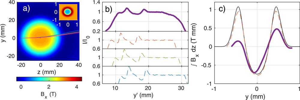
We start by considering how protons of different energies passing through a significant background magnetic field are deflected by different angles depending on their energies, such as shown in Fig. 1(a). This results in a succession of different radiographs from protons of different energies, imprinted one on the other, each shifted by a small distance, as shown in Fig. 1(b). This plot shows proton radiographs calculated for the example magnetic field profile (with no electric fields) at three different distinct energies, from 10 to 14 MeV, with each monoenergetic radiograph slightly displaced because of the background magnetic field. Each layer of RCF absorbs protons over a finite range of energies, and so, when the proton beam has a broadband energy spectrum, the radiographs measured by each separate layer of film are all blurred in the direction of proton deflection.
![]()
Figure 1.(a) Example of the magnetic field structure, with a large background field surrounding a millimeter-scale signal region near the center (a close-up of which is shown in the inset on the top right). Overlaid are the paths of monoenergetic proton beams of energies 10 MeV (blue), 16 MeV (yellow), and 21 MeV (pink). (b) Example of three synthetic monoenergetic radiographs (dashed lines) at 10 MeV (blue), 12 MeV (green), and 14 MeV (red), compared with a composite combined radiograph (solid purple), modeled using a thermal proton distribution absorbed by a layer of RCF. (c) Magnetic field profile reconstructed from the combined blurred radiograph (bold purple line) compared with the true field profile (solid black) and the reconstruction from the monoenergetic radiograph at 14 MeV (dashed red).
In this example, the background field was chosen to resemble the conditions of a recent experiment. The peak field strength of 3 T along the x direction extends over a diameter of around 40 mm, as shown in Fig. 1(a), with the proton beam initially traveling along the z axis and experiencing a total integrated field of ∫Bx dz ≈ 90 T mm; the proton beam is therefore deflected in the y direction. The synthetic radiograph intensities were calculated using the EPOCH particle-in-cell code19 and measured at an RCF position 100 mm from the origin. The radiographs were combined, weighted by a thermal proton spectrum at T = 5 MeV and by the calculated absorption of an RCF layer with an absorption peak at 10.6 MeV and a full width at half maximum of 0.4 MeV. Note that this blurring is asymmetric and changes both the shape and the symmetry properties of the final radiograph. Using this combined radiograph to reconstruct the magnetic field profile therefore gives a poor estimate, as shown in Fig. 1(c). The amplitude of the signal reconstructed from the combined radiograph is much lower than the true value, as though the radiograph had been taken with very poor spatial resolution. The shape of the profile is also distinctly different owing to the asymmetric blurring. The reconstruction using a monoenergetic radiograph, on the other hand, is close to the true field, showing that the discrepancy arises from the blurring rather than from the reconstruction. To calculate the degree of blurring in these synthetic radiographs, we can consider each component in turn.
A. Proton deflection
First, we can calculate the deflection of protons in a known background magnetic field by tracking the path of the proton through the field, as shown in Fig. 1(a). In experiments, however, if the background field is not well characterized, the deflection must normally be calibrated using a known fiducial. By placing a wire at the interaction point and taking measurements of the position of its shadow on different layers of RCF, we can estimate the vertical displacement of the beam on the stack
![]()
Figure 2.(a) Deflection of the proton beam vs energy, measured by tracking the edge of the proton distribution in synthetic radiographs, and fitted to
B. Protons absorbed
Second, the energies deposited into the RCF stack by the proton beam can be calculated using a finite element opacity model, where for a number of protons N(E, z) of a given energy E and depth in the stack z, the absorption in the stack is given by dN(E, z) = −σ(E, z)N(E, z)dz for an opacity σ(E, z). σ can be tabulated against proton energy for different materials, with opacity higher for denser materials and for lower proton energies. The proton populations through the RCF stack can be calculated by integration as log[N(E, z)/N0(E)] = −∫σ(E, z)dz, for an initial proton energy spectrum N0(E). The response function for a given slice of RCF labeled i with thickness ti is then Ri(E) = [N(E, zi) − N(E, zi + ti)]/N0(E). These response functions are plotted in Fig. 2(b), showing the characteristic Bragg peaks. For each layer of RCF, this results in a negligible response at low energies (where almost all the protons have already been deposited earlier in the stack), followed by a sudden spike in absorption at a particular energy (where the integrated opacity is close to 1), followed by a decay in response at higher energies (where the integrated opacity remains much less than 1).
C. Proton spectrum
Finally, the response curves, which vary for each layer in the RCF stack, should then be weighted by the energy distribution of the proton beam, N0(E), which is the same for all layers but varies from shot to shot. The spectrum is generally estimated using the dose measured on each piece of RCF, compared with the proton energy most strongly absorbed by each layer. Either fitting to an expected spectral shape [e.g., a thermal spectrum given by N0(E) ∝ e−E/T for a temperature T] or interpolating between these measured points on the spectrum then gives an estimate of the proton energy distribution, with examples from two different laser shots shown in Fig. 2(c) with estimated temperatures of 4.8 and 5.7 MeV. Strictly speaking, however, each layer of RCF absorbs protons from a range of energies, as we saw, and the proton spectrum should be found self-consistently, finding a spectrum N0(E) such that the measured dose on each slice i is Di = ∫Ri(E)N0(E)dE. This can be approached by inversion or iteratively, starting at the back of the RCF stack where the response is only due to high energies and Ri(E) is mostly zero.
III. BLURRING AS A CONVOLUTION
Now we understand the causes of blurring in proton radiographs taken through a strong background magnetic field, we can work to remove the effect and recover an estimate of what the radiographs would look like without the background field. If the proton energy is conserved, then, in the absence of electric fields, the deflection of protons depends on the path-integrated magnetic field as
On the other hand, the intensity of the proton radiograph is dependent on the gradient of the deflection. A one-dimensional radiograph has an intensity profile given by I/I0 = |∂y′/∂y|−1, where y is the position of protons as they pass through the object plane at z = 0, and y′ is the position of protons as they arrive at the RCF stack. This means that the relevant quantity for the intensity profile is
Next, we assume that over the energy range of protons absorbed by a single layer of RCF, the radiograph is identical. Generally, lower-energy protons are deflected more by the magnetic fields, giving radiographs with higher variations in intensity and more caustic features. At low proton energies or strong fields, the assumption of identical radiographs over a small energy range is therefore not accurate. Where each RCF layer is only absorbing protons from a relatively narrow energy spread, however, we can write the intensity profile from protons of a given energy on a given shot as
When these protons are absorbed by a given RCF layer i, they produce a measured dose shape of the form
Furthermore, if the contrast of the radiograph is not so high as to form caustic features (i.e., I/I0 − 1 ≪ 1), then we can generalize this convolution kernel to any RCF position or proton source location. If there is a direct mapping between points in the object plane described by the coordinate y and points on the RCF stack described by
Some examples of convolution kernels are shown in Fig. 3(a), calculated using the measured deflection and RCF response functions shown in Fig. 2 and the thermal proton energy spectra at T = 5 MeV and T = 10 MeV, and plotted vs position in the object plane. For the first RCF layer at the front of the stack, with proton energies around 5 MeV, the proton deflection is large, and the resulting blurring kernel has a broad tail to the left of the ideal monoenergetic peak. This would blur out any magnetic field features smaller than a few millimeters. By the fourth RCF layer in the stack, however, with proton energies around 15 MeV, the effect of blurring occurs over less than a millimeter.
![]()
Figure 3.(a) Examples of convolution kernels calculated for different RCF layers for a
Comparing the results for a proton spectrum with T = 10 MeV, the broader energy range of protons incident on the RCF stack here results in broader blurring kernels. There is therefore a trade-off with proton energy: for higher-energy protons, deflection is small and blurring is negligible, but the dose absorbed in the RCF is lower, and the amplitude of the signal will also be smaller. Increasing the dose by obtaining higher-temperature proton spectra will also increase the effect of blurring.
We can compare the effective spatial resolutions by looking at the standard deviations of the convolution kernels, plotted in Fig. 3(b) vs the mean proton energy absorbed by each layer of the RCF stack. This shows the reduction in the kernel width with proton energy, such that for a 3 T background field with a field integral of 90 T mm, the blurring width changes from around 2 mm in the object plane at 5 MeV to under 250 µm above 20 MeV. Increasing the temperature of the proton beam to 10 MeV could increase the proton dose at these higher energies, but would also lead to an increase in the blurring width by around 50%. If the field strength is increased to 10 T, on the other hand, the effect of blurring is very significant, even at these higher energies, with a blurring width of 1 mm in the object plane at 20 MeV. Whereas magnetized plasma experiments that employ proton radiography often attempt to increase the proton temperature or the magnetic field strength, both of these changes will lead to greater blurring, and great care must be taken if small features in the magnetic field are to be measured.
IV. DECONVOLUTION
Having expressed the blurring as a linear convolution, we can perform a deconvolution and recover the monoenergetic radiograph f(y′; E0) from the measured dose profile. There are several possible deconvolution algorithms, of which we use the Richardson–Lucy technique20,21 for its stability. Figure 4(a) shows the same combined radiograph described earlier, calculated from a thermal proton spectrum with T = 5 MeV incident on a layer of RCF after passing through a background magnetic field with a strength of 90 T mm, as shown in Fig. 1. This radiograph is compared with the 10 MeV monoenergetic radiograph predicted from particle-in-cell simulations and with the estimated radiograph recovered using deconvolution of the combined radiograph. This shows how the deconvolution increases the contrast of the radiograph, with the result closely approximating the profile of the monoenergetic radiograph. Under these conditions, this therefore makes the recovered magnetic field profile more accurate after deconvolution has been used, as shown in Fig. 4(b). The deconvolved radiograph gives an estimate of the magnetic field that is almost an exact match to the true profile for |r| > 0.3 mm, with the same symmetry and amplitude. On-axis, however, the deconvolution leads to an exaggeration of the magnetic field strength and a significant error, demonstrating that this deconvolution is a useful tool, but not a perfect solution to the problem of blurring.
![]()
Figure 4.(a) Synthetic radiographs from a thermal proton beam passing through a background field with a strength of 90 T mm before being absorbed by a layer of RCF. The combined radiograph (purple line) and that after application of deconvolution (dash-dotted red line) are compared with a monoenergetic radiograph at a proton energy of 10 MeV (solid blue). (b) Reconstructed magnetic field profile recovered from the synthetic radiographs. Again, the result without deconvolution (purple line) and the result using deconvolution (dash-dotted red line) are compared with the true magnetic field profile (solid black line).
Deconvolution of a blurred radiograph clearly has limitations, and cannot perfectly recover a monoenergetic radiograph or the true magnetic field profile. First, applying any deconvolution algorithm to real data can amplify noise features, such as can be seen on the right of Fig. 4(a); instead of a flat I = I0 profile there is an artifact from the application of a deconvolution to noise. This can lead to inaccurate field reconstructions away from the main features, or where the amplitude of the noise is similar to that of the signal. Second, the shape of the radiograph is not identical for different proton energies, with the greater deflection of lower-energy protons leading to a higher-contrast radiograph. By assuming that the radiograph shape is constant, the deconvolved signal will tend to overestimate the amplitude of the magnetic field profile. Finally, the deconvolution process is only an estimate of the true deconvolution, and cannot perfectly recover the original signal. The broader the convolution kernel relative to the feature size of the signal, the more poorly will the deconvolution algorithm perform. All of these limitations mean that deconvolution is more helpful in estimating the true magnetic field profile under some conditions than others.
We can study the accuracy of the deconvolution under different conditions by simulating the blurring process and the deconvolution. Figure 5(a) shows an example of an arbitrary integrated magnetic field profile (solid black line), defined here as a sinusoid with a linearly increasing amplitude. The blurring is modeled by calculating a series of synthetic radiographs with different proton energies, before displacing the radiographs by the deflections shown in Fig. 2(a). This assumes that the background field is constant over the signal region and does not change the shape of the radiograph. The proton source is point-like in these ideal synthetic radiographs, with the spatial resolution limited only by the grid size of 2 µm. The absorption of protons in the third layer of RCF is then modeled using a thermal proton spectrum with a temperature of 5 MeV and an RCF response curve as shown in Fig. 2(b). This results in significant blurring of the recovered magnetic field profile (dashed blue line), with the amplitude of the sinusoid reduced by around a factor of three. Applying a deconvolution algorithm, however, with a convolution kernel such as shown in Fig. 3(a), recovers a sharp radiograph. This gives an estimate of the magnetic field that closely matches the original profile.
![]()
Figure 5.(a) Arbitrary integrated magnetic field profile with a scale length of 0.5 mm (solid black line) compared with an example of a reconstructed field from a blurred radiograph (dashed blue line) and after deconvolution (dash-dotted red line). (b) Accuracy of the reconstruction before (dashed lines) and after (solid lines) deconvolution, plotted vs the mean proton energy absorbed in each layer of RCF, shown for thermal
Figure 5(b) shows how, under different conditions, the accuracy of the magnetic field reconstruction varies depending on the RCF layer, with layers that absorb higher-energy protons measuring less blurring and giving a lower error. The error is shown as the root-mean-square (rms) difference in integrated magnetic field, relative to the rms of the original integrated magnetic field profile. Whereas the blurred radiographs (dashed lines) give relative errors of around 50% or more, the error after applying the deconvolution (shown by the solid lines) falls to under 10%. The deconvolution is not perfect, however, and for the first layer in the RCF stack, absorbing proton energies around 5 MeV, the relative error after deconvolution is still around 50%. At these low proton energies, the large widths of the kernels make the deconvolution inaccurate, while the shape of the radiograph also changes rapidly with proton energy and the blurring is not described well by a convolution. We can therefore establish first that applying a deconvolution with the relevant kernel substantially improves the accuracy of reconstructing the magnetic field, and second that this deconvolution performs better at higher proton energies, above 10 MeV.
By changing the modeled deflection and proton spectrum, we can also explore how the strength of the background field and the temperature of the proton beam affect the accuracy of the reconstruction. As expected, and in agreement with Fig. 3(b), both a higher background field and a higher-temperature proton beam cause greater blurring and a reduction in accuracy of the reconstruction, both before and after the application of deconvolution. Whereas increasing the proton beam temperature from 5 MeV (shown by the blue lines) to 10 MeV (red lines) makes the relative error without any deconvolution around 10% worse, the main effect on the deconvolution process is to increase the proton energy required for an accurate reconstruction. A higher proton temperature not only increases the width of the smearing kernel, but also weakens the assumptions of a linear convolution. The shape of the radiograph can vary considerably over the larger energy range, making the deconvolution inaccurate below 15 MeV. Above this point, however, the assumptions hold and the kernel is narrower, making the deconvolution accurate to better than 10%.
Similarly, increasing the background field strength from 90 to 300 T mm (shown by the purple lines) makes the convolution kernels much broader, and increases the relative error of the blurred reconstruction by around 20%. The kernels for RCF layers at the front of the stack have widths greater than 2 mm in the object plane, as shown in Fig. 3(b), and it is therefore unsurprising that the deconvolution cannot accurately recover the features of the true magnetic field profile. By RCF layers deeper in the stack absorbing higher proton energies, on the other hand, the deconvolution accurately reproduces the true magnetic field profile, with a relative error of less than 10% for proton energies greater than 20 MeV. In this way, accurately probing magnetic fields in the presence of a strong background field requires high doses of high-energy protons, but unfortunately using high-temperature proton beams to achieve this can be counterproductive. Deconvolution is very successful at recovering the signal magnetic field profile even when blurring is severe, but spatial features that are too small are lost—a feature that we explore in detail next.
We can estimate the spatial resolution of the deconvolved radiographs by calculating the radiograph and the reconstructed magnetic field profile as before, now using a series of magnetic field profiles with the same form as shown in Fig. 5(a) but with wavelengths from 16 mm down to 12.5 µm. For each layer of RCF, the smallest wavelength is found that still gives less than 10% rms error. The accuracy of the blurred radiographs, on the other hand, is estimated using the convolution kernel by finding the wavenumber where the Fourier transform of the relevant kernel falls to 90% of the maximum amplitude, thereby introducing a 10% error in the corresponding wavelength.
The resulting estimates of the spatial resolution in the object plane are shown in Fig. 5(c), with the maximum spatial resolution that can be recovered with an accuracy of better than 10% plotted vs proton energy for synthetic radiographs, both before and after the application of deconvolution, and for different background magnetic field strengths. This shows how the blurring strongly limits the spatial resolution, with this effect being worse at lower proton energies, but still problematic for proton energies above 20 MeV. At 20 MeV, the spatial resolution is limited to around a millimeter for a background field strength of 30 T mm, but around 10 mm for a background field strength of 300 T mm.
Applying the deconvolution improves the spatial resolution above 10 MeV by around an order of magnitude. For a 30 T mm background field, spatial resolutions of tens of micrometers in the object plane are achievable for proton energies higher than 20 MeV. The deconvolution is not perfect and cannot recover all of the lost resolution, with the front layers of the RCF stack experiencing little benefit when absorbing protons around 10 MeV and below. Higher proton energies, which experience less deflection, again correspond to better spatial resolution. For the strongest 300 T mm background field, the spatial resolution even after using deconvolution is around a millimeter at 15 MeV, or 300 µm at 25 MeV. When using a proton source with a broad energy spread to conduct radiography in applied magnetic fields, increasing the magnetic field strength will reduce the spatial resolution achievable, even after using deconvolution.
V. CONCLUSIONS
We have extended proton probing to a new class of experiments that use applied magnetic fields surrounding the region of interest. These experiments encounter significant difficulties, because not only is the proton beam deflected by the background field, but this deflection is energy-dependent. When combined with a broadband proton energy spectrum and absorption in layers of RCF, this deflection results in significant blurring of the proton radiograph. This blurring is most severe for layers of RCF at the front of the stack, which absorb lower-energy protons, but is also a significant problem for protons of higher energies, above 20 MeV for the conditions considered here. Furthermore, increasing the temperature of the proton beam to access higher proton energies will itself worsen the effect of blurring.
However, we have also shown that under certain conditions, the blurring can be modeled as a linear convolution and removed using a deconvolution algorithm. When the background field is large and slowly varying in space compared with the signal, and the relative energy spread of protons absorbed by the RCF is sufficiently small, we can therefore recover a good estimate for a monoenergetic radiograph and accurately reconstruct the magnetic field that we wish to measure, despite the presence of a strong background field. By looking at how the convolution kernel changes with the background field strength, the proton temperature, and the RCF absorption, we can estimate the loss of spatial resolution caused by the blurring and calculate the deconvolution required.
We have shown how deconvolution substantially increases the accuracy of the reconstructed magnetic field profile, with the error in the reconstruction falling from over 50% to under 10%, and the spatial resolution of the radiographs is improved by an order of magnitude. While no estimate of the true magnetic field profile will be perfect, calculating the kernel and applying deconvolution allows us to recover much greater spatial resolution than is possible from the blurred radiographs, down to around 100 µm for a 90 T mm background field. We have in this way extended the power of proton radiography to experiments with applied magnetic fields, allowing researchers to study changes to electric and magnetic fields even under these challenging experimental conditions.
SUPPLEMENTARY MATERIAL
ACKNOWLEDGMENTS
Acknowledgment. The authors are grateful for the support of LLNL Academic Partnerships (Grant No. B618488), EUROfusion Enabling Research Grant Nos. AWP17-ENR-IFE-CCFE-01 and AWP17-ENR-IFE-CEA-02, and UK EPSRC Grant Nos. EP/P026796/1 and EP/R029148/1.
References
[1] M.Borghesi, S. V.Bulanov, J.Fuchs, A. J.MacKinnon, P. K.Patel, M.Roth. Fast ion generation by high-intensity laser irradiation of solid targets and applications. Fusion Sci. Technol., 49, 412-439(2006).
[2] N. L.Kugland, H.-S.Park, C.Plechaty, J. S.Ross, D. D.Ryutov. Invited article: Relation between electric and magnetic field structures and their proton-beam images. Rev. Sci. Instrum., 83, 101301(2012).
[3] A. F. A.Bott, G.Gregori, M. F.Kasim, D. Q.Lamb, P.Tzeferacos, S. M.Vinko. Retrieving fields from proton radiography without source profiles. Phys. Rev. E, 100, 033208(2019).
[4] S.Bandyopadhyay, A. E.Dangor, R. G.Evans, P.Fernandes, M. G.Haines, M. C.Kaluza, C.Kamperidis, R. J.Kingham, K.Krushelnick, S.Minardi, Z.Najmudin, P. M.Nilson, M.Notley, C. P.Ridgers, W.Rozmus, M.Sherlock, M.Tatarakis, A. G. R.Thomas, M. S.Wei, L.Willingale. Fast advection of magnetic fields by hot electrons. Phys. Rev. Lett., 105, 095001(2010).
[5] P. A.Amendt, R.Betti, J. A.Frenje, J.Hund, J. D.Kilkenny, O. L.Landen, C. K.Li, A. J.Mackinnon, M. J.-E.Manuel, D. D.Meyerhofer, A.Nikroo, R. D.Petrasso, H. G.Rinderknecht, M. J.Rosenberg, F. H.Séguin, N.Sinenian, J. M.Soures, R. P. J.Town, S. C.Wilks, A. B.Zylstra. Proton imaging of hohlraum plasma stagnation in inertial-confinement-fusion experiments. Nucl. Fusion, 53, 073022(2013).
[6] L.Antonelli, A. F. A.Bott, P. T.Campbell, D. C.Carroll, G.Gregori, J.Halliday, Y.Katzir, P.Kordell, K.Krushelnick, S. V.Lebedev, Y.Ma, E.Montgomery, M.Notley, C. A. J.Palmer, C. P.Ridgers, A. A.Schekochihin, M. J. V.Streeter, A. G. R.Thomas, E. R.Tubman, L.Willingale, N.Woolsey. Field reconstruction from proton radiography of intense laser driven magnetic reconnection. Phys. Plasmas, 26, 083109(2019).
[7] M.Borghesi, A. F. A.Bott, B.Coleman, G.Cooper, C. N.Danson, P.Durey, J. M.Foster, P.Graham, G.Gregori, E. T.Gumbrell, M. P.Hill, T.Hodge, A. S.Joglekar, S.Kar, R. J.Kingham, M.Read, C. P.Ridgers, J.Skidmore, C.Spindloe, A. G. R.Thomas, P.Treadwell, E. R.Tubman, L.Willingale, S.Wilson, N. C.Woolsey. Observations of pressure anisotropy effects within semi-collisional magnetized plasma bubbles. Nat. Commun., 12, 334(2021).
[8] A.Baird, A. R.Bell, A.Benuzzi-Mounaix, R.Bingham, C.Constantin, R. P.Drake, M.Edwards, E. T.Everson, G.Gregori, C. D.Gregory, M.Koenig, Y.Kuramitsu, W.Lau, F.Miniati, J.Mithen, C. D.Murphy, C.Niemann, H.-S.Park, A.Ravasio, B. A.Remington, B.Reville, A. P. L.Robinson, D. D.Ryutov, Y.Sakawa, K.Schaar, N. C.Woolsey, S.Yang. Generation of scaled protogalactic seed magnetic fields in laser-produced shock waves. Nature, 481, 480-483(2012).
[9] A. R.Bell, R.Bingham, R.Crowston, H. W.Doyle, R. P.Drake, M.Fatenejad, G.Gregori, M.Koenig, Y.Kuramitsu, C. C.Kuranz, D. Q.Lamb, D.Lee, M. J.MacDonald, J.Meinecke, F.Miniati, C. D.Murphy, H.-S.Park, A.Pelka, A.Ravasio, B.Reville, Y.Sakawa, A. A.Schekochihin, A.Scopatz, P.Tzeferacos, W. C.Wan, N. C.Woolsey, R.Yurchak. Turbulent amplification of magnetic fields in laboratory laser-produced shock waves. Nat. Phys., 10, 520-524(2014).
[10] D. T.Blackfield, S. A.Hawkins, D. D.-M.Ho, B. G.Logan, L. J.Perkins, M. A.Rhodes, D. J.Strozzi, G. B.Zimmerman. The potential of imposed magnetic fields for enhancing ignition probability and fusion energy yield in indirect-drive inertial confinement fusion. Phys. Plasmas, 24, 062708(2017).
[11] B. D.Appelbe, J. P.Chittenden, A.Crilly, K.McGlinchey, J. K.Tong, C. A.Walsh, M. F.Zhang. Perturbation modifications by pre-magnetisation of inertial confinement fusion implosions. Phys. Plasmas, 26, 022701(2019).
[12] S. A.Slutz, R. A.Vesey. High-gain magnetized inertial fusion. Phys. Rev. Lett., 108, 025003(2012).
[13] J. M.Koning, M. M.Marinak, K. J.Peterson, A. B.Sefkow, D. B.Sinars, S. A.Slutz, R. A.Vesey. Design of magnetized liner inertial fusion experiments using the Z facility. Phys. Plasmas, 21, 072711(2014).
[14] R.Betti, P. Y.Chang, G.Fiksel, M.Hohenberger, J. P.Knauer, F. J.Marshall, D. D.Meyerhofer, R. D.Petrasso, F. H.Séguin. Fusion yield enhancement in magnetized laser-driven implosions. Phys. Rev. Lett., 107, 035006(2011).
[15] R.Betti, P.-Y.Chang, G.Fiksel, M.Hohenberger, J. P.Knauer, F. J.Marshall, D. D.Meyerhofer, R. D.Petrasso, F. H.Séguin. Inertial confinement fusion implosions with imposed magnetic field compression using the OMEGA laser. Phys. Plasmas, 19, 056306(2012).
[16] P. X.Belancourt, H.Chen, R. P.Drake, J. R.Fein, A. U.Hazi, P. A.Keiter, S. R.Klein, C. C.Kuranz, M. J.MacDonald, M. J.-E.Manuel, J.Park, B. B.Pollock, A. M.Rasmus, M. R.Trantham, G. J.Williams, R. P.Young. Experimental results from magnetized-jet experiments executed at the Jupiter Laser Facility. High Energy Density Phys., 17, 52-62(2015).
[17] B.Albertazzi, J. M.Bonnet-Bidaud, F.Brack, E.Brambrink, J. E.Cross, R. P.Drake, E.Falize, E.Filippov, G.Gregori, R.Kodama, M.Koenig, F.Kroll, C. C.Kuranz, D.Lamb, C.Li, P.Mabey, M. J.-E.Manuel, T.Morita, M.Mouchet, N.Ozaki, A.Pelka, S.Pikuz, Y.Sakawa, U.Schramm, P.Tzeferacos, L.Van Box Som, R.Yurchak. Experimental platform for the investigation of magnetized-reverse-shock dynamics in the context of POLAR. High Power Laser Sci. Eng., 6, e43(2018).
[18] L.Antonelli, N.Booth, P.Bradford, D.Carroll, R. J.Clarke, M.Ehret, K.Glize, R.Heathcote, M.Khan, J. D.Moody, S.Pikuz, B. B.Pollock, M. P.Read, C. P.Ridgers, S.Ryazantsev, J. J.Santos, C.Spindloe, V. T.Tikhonchuk, N. C.Woolsey. Proton deflectometry of a capacitor coil target along two axes. High Power Laser Sci. Eng., 8, e11(2020).
[19] T. D.Arber, A. R.Bell, K.Bennett, C. S.Brady, R. G.Evans, P.Gillies, A.Lawrence-Douglas, M. G.Ramsay, C. P.Ridgers, H.Schmitz, N. J.Sircombe. Contemporary particle-in-cell approach to laser-plasma modelling. Plasma Phys. Controlled Fusion, 57, 113001(2015).
[20] W. H.Richardson. Bayesian-based iterative method of image restoration. J. Opt. Soc. Am., 62, 55-59(1972).
[21] L. B.Lucy. An iterative technique for the rectification of observed distributions. Astron. J., 79, 745(1974).


Set citation alerts for the article
Please enter your email address

© Copyright 2018-2021 | Chinese Laser Press. All Rights Reserved 沪ICP备15018463号-20