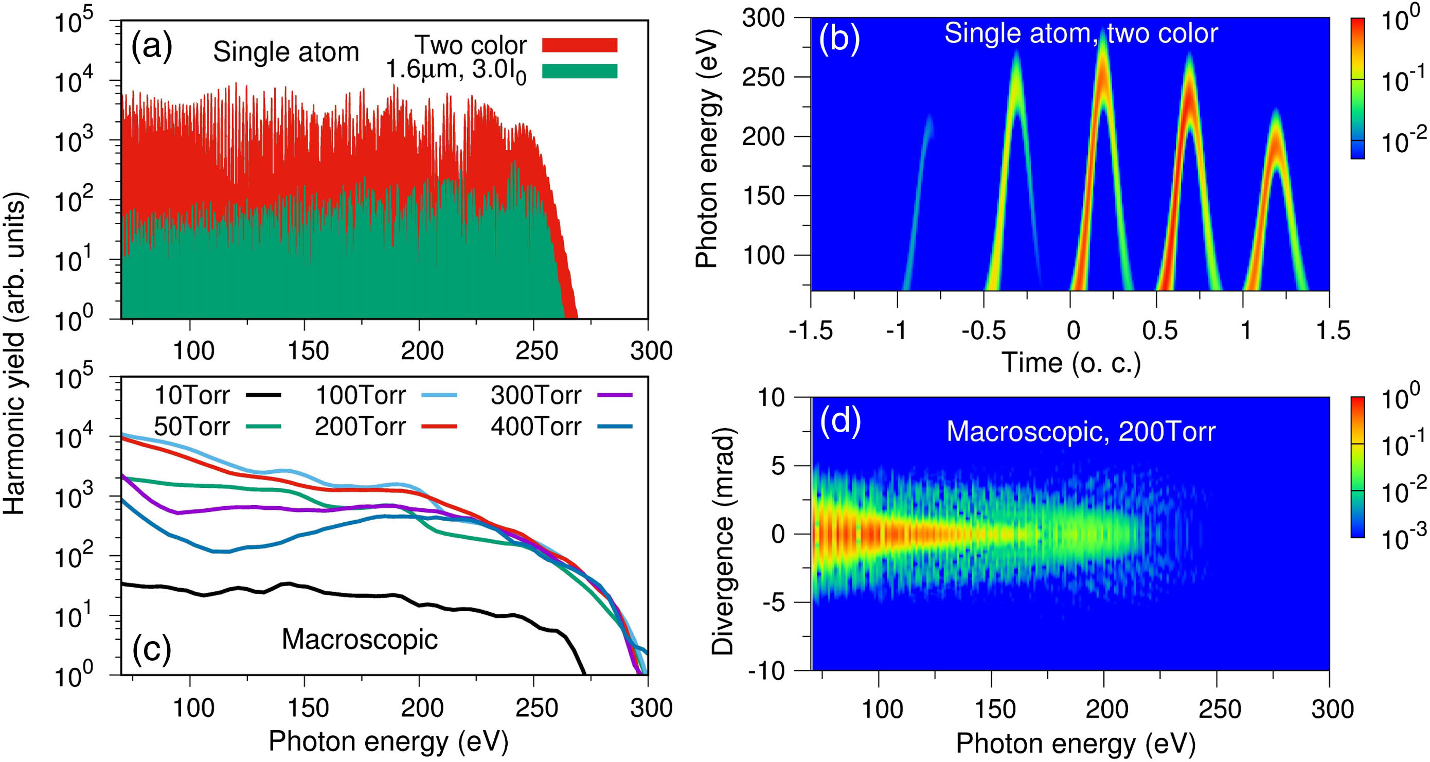
Fig. 1. (a) Single-atom harmonic yields with a 1.6-μm and a two-color laser pulse. The corresponding time-frequency harmonic emissions by the two-color pulse are shown in (b). (c) Macroscopic harmonic spectra (integrated over the exit plane of the gas cell and smoothed by using Bezier curve) generated by the two-color laser pulse at different gas pressures. Optimal pressure for the highest harmonic yields and the largest cutoff energy was found to be 200 Torr. The angular divergence of the far-field harmonic generated at this pressure is shown in (d). See text for other laser parameters.

Fig. 2. (a) Evolution of harmonic spectra against the propagation distance by a two-color laser pulse at the gas pressure of 400 Torr. The propagation distances are as indicated. (b) The harmonic spectrum at the exit of the gas cell calculated including both dispersion and absorption effects (w/dis+abs) is compared with calculations where only absorption (only abs) is included, and with calculations where neither absorption nor dispersion (no dis+abs) is included. The absorption length versus harmonic energy for gas pressure at 400 Torr from NIST [56] is also plotted (see right-hand scale). (c), (d) Time-frequency analysis of the harmonic emissions (normalized) at r=11  μm of the exit plane. The optical cycle (o.c.) is defined with respect to the fundamental 1.6-μm laser.

Fig. 3. Time-frequency analysis of the harmonic emissions (normalized) at r=11  μm at different propagation planes for the gas pressure of 400 Torr including both dispersion and absorption effects. The optical cycle (o.c.) is defined with respect to the fundamental 1.6-μm laser.

Fig. 4. Evolution of macroscopic two-color harmonic spectra with the propagation distance (as indicated) for two gas pressures: (a) 50 Torr and (b) 200 Torr. (c), (d) Time-frequency analysis of macroscopic harmonic emissions (normalized) at r=11  μm of the exit plane.

Fig. 5. Time-dependent electric fields of the two-color laser pulse at r=11  μm for three gas pressures (a) 50 Torr, (b) 200 Torr, and (c) 400 Torr at three positions: d=0  mm (at the entrance), d=1  mm (in the middle), and d=2  mm (at the exit plane of the gas cell), respectively. Enlarged figures of the electric fields are shown for the two time intervals, one at the leading edge and the other at the trailing edge of the pulse. Note that the driving field has been substantially weakened due to the geometric phase, the dispersion, and the plasma dispersion as the beam travels in space and time in the gas cell.

Fig. 6. Time-frequency analysis of harmonic emission driven by the electric field at d=1  mm for an off-axis position, r=11  μm (shown in Fig. 5) for three gas pressures: (a) 50 Torr, (b) 200 Torr, and (c) 400 Torr. The 120 eV harmonic emissions are lined out from (a)–(c) and replotted in (d) for the three pressures at d=1  mm. The same plots are shown at (e) d=1.5  mm and (f) d=2  mm. One observes that each harmonic burst of “short”-trajectory electron emission changes in time depending on the gas pressure as well as the propagation distance.

Fig. 7. Macroscopic harmonic spectra (smoothed by using Bezier curve for easy comparison) generated by (a) two-color and (b) 1.6-μm laser pulses at different gas pressures.

Fig. 8. Harmonic emission (normalized at the highest peak in each figure) in the far field using the optimized two-color laser pulses. (a)–(c) are for the generation of optimal harmonics, and (d)–(f) are for the generation of suppressed harmonics. The beam waists of the 1.6-μm laser in the two-color waveforms are indicated on top of the figures. Other parameters for (a)–(f) are listed in Table 2.

Fig. 9. Total harmonic yields integrated over the radial dimension under the (a) optimal and (b) suppression conditions. Panels (a) and (b) correspond to harmonic emissions in Figs. 8(a)–8(c) and in Figs. 8(d)–8(f), respectively. In both (a) and (b), the ratio of the harmonic yield between top, middle, and bottom curve is 16∶4∶1.

Table 1. Laser Parameters for a Two-Color Laser Pulse^a

Table 2. Macroscopic Parameters for Harmonic Emissions in Fig. 8^a