
Shaoyu Wang, Weiwen Wu, Changcheng Gong, Fenglin Liu. Study of Parallel Translation Computed Laminography Imaging[J]. Acta Optica Sinica, 2018, 38(12): 1211002
- Acta Optica Sinica
- Vol. 38, Issue 12, 1211002 (2018)
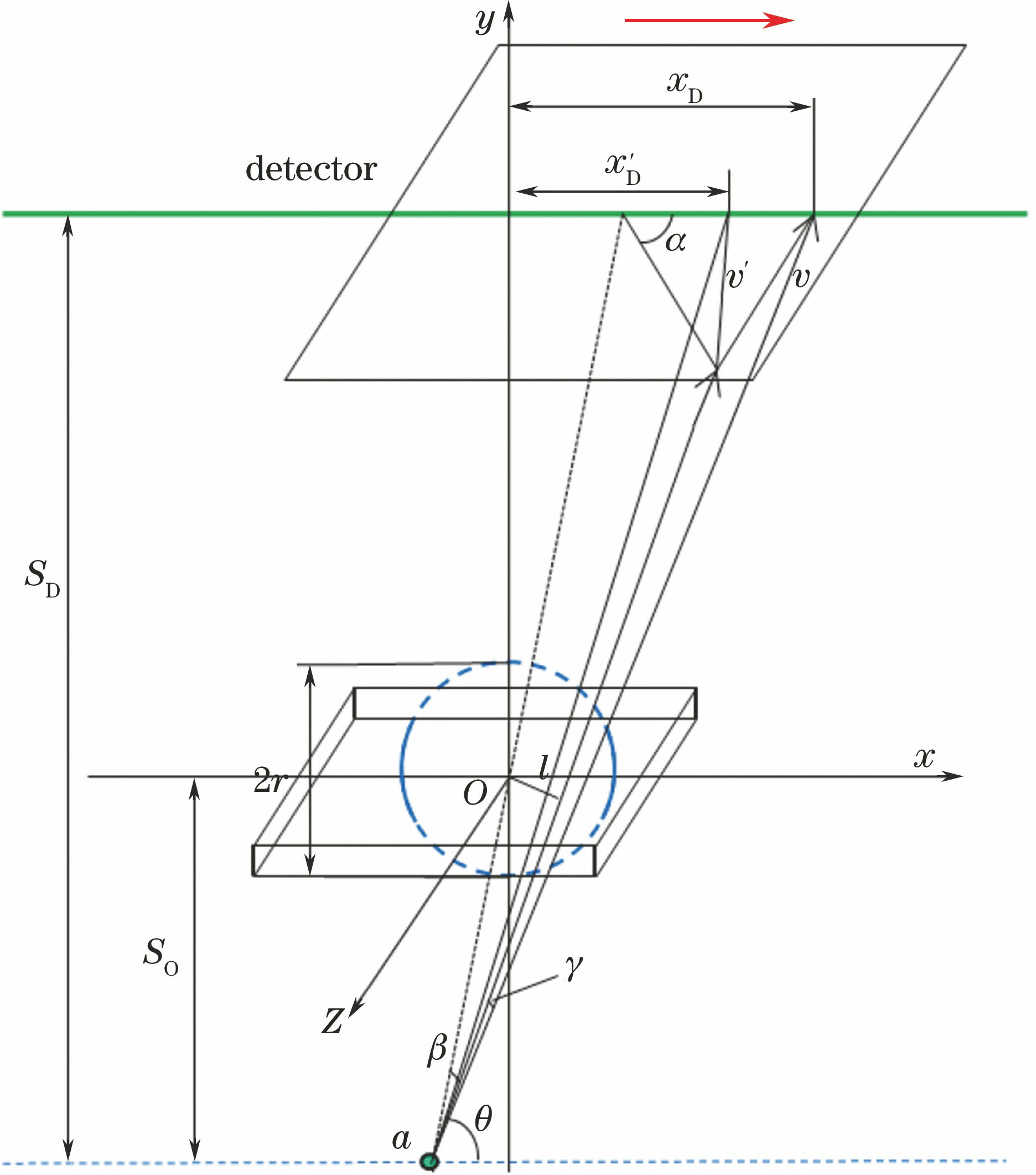
Fig. 1. Imaging geometry and variables of PTCL system
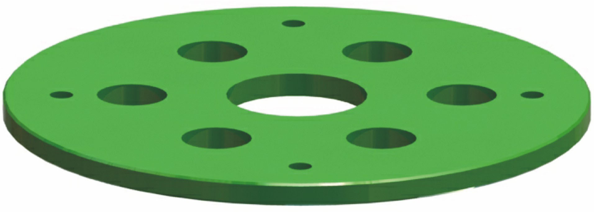
Fig. 2. Simulation phantom
Fig. 3. 120° limited angle of global reconstructed images from noise-free cone-beam data. (a) Three-dimensional display; (b) 110th longitudinal profile, the display window is [0 0.8]
Fig. 4. 130th slice of global reconstructed images from noise-free cone-beam data. (a)-(d) FDK algorithm; (e)-(h) SART algorithm; (i)-(l) SART+TV algorithm, respectively. The first to fourth columns are from 30°, 60°, 90° and 120° limited angle, respectively, the display window is [0 0.8]
Fig. 5. Central horizontal profiles of global reconstructed images from noise-free cone-beam data by (a) FDK, (b) SART and (c) SART+TV algorithm
Fig. 6. 130th slice of global reconstructed images from noise cone-beam data. (a)-(d) FDK algorithm; (e)-(h) SART algorithm; (i)-(l) SART+TV algorithm, respectively. The first to fourth columns are from 30°, 60°, 90° and 120° limited angle, respectively, the display window is [0 0.8]
Fig. 7. Central horizontal profiles of 130th slice global reconstructed images from noise cone-beam data by (a) FDK, (b) SART and (c) SART+TV algorithm
Fig. 8. 12th slice of local reconstructed images from noise-free cone-beam data. (a)-(d) FDK algorithm; (e)-(h) SART algorithm; (i)-(l) SART+TV algorithm, respectively. The first to fourth columns are from 30°, 60°, 90° and 120° limited angle, respectively, the display window is [0 1.5]
Fig. 9. Horizontal profiles along y=14 within 12th slice of local reconstructed image from noise-free cone-beam by (a) FDK,(b) SART and (c) SART+TV algorithm
Fig. 10. Reconstructed images from noise-free cone-beam and 60° projection angle with different magnification ratios by using SART+TV algorithm. (a) Magnification ratio is 8.89; (b) magnification ratio is 6, the display window is [0 1.5]
Fig. 11. Horizontal profiles along y=14 of 12th slice reconstructed images with 60° limited angle and noise-free cone-beam data by SART+TV algorithm
Fig. 12. (a) Convergence curve of noise-free cone-beam data with 60° limited angle by using SART+TV algorithm; (b) enlarged image of Fig. (a)
Fig. 13. (a) Detected chip; (b) PCB
Fig. 14. 128th slice reconstructed images by using (a) FDK and (b) SART+TV methods
Fig. 15. PCB 111th slice reconstructed results by using (a) FDK and (b) SART+TV methods
|
Table 1. Parameters of the numerical simulation
|
Table 2. Normalized mean square error of global reconstructed images from noise-free cone-beam data with different angles and different algorithms10-4
|
Table 3. Normalized mean square error of global reconstructed images from noise cone-beam data with different angles and different algorithms10-4
|
Table 4. Quantitative assessment in terms of local reconstruction images normalized mean square error10-4
|
Table 5. Scanning parameters

Set citation alerts for the article
Please enter your email address
© Copyright 2018-2021 | Chinese Laser Press. All Rights Reserved 沪ICP备15018463号-20