
Kangjun Zhao, Chenxin Gao, Xiaosheng Xiao, Changxi Yang, "Real-time collision dynamics of vector solitons in a fiber laser," Photonics Res. 9, 289 (2021)
- Photonics Research
- Vol. 9, Issue 3, 289 (2021)
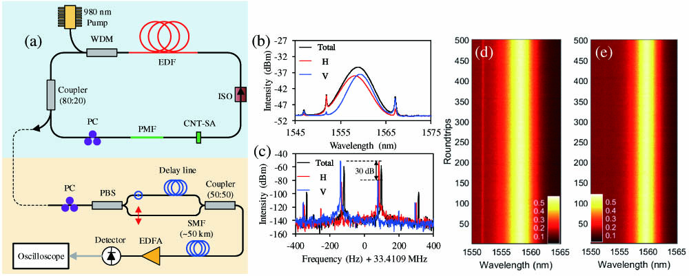
Fig. 1. Generation and characterization of two vector solitons with slightly different repetition rates from a mode-locked fiber laser. (a) Schematic of the mode-locked fiber laser (blue) and single-shot spectral measurement (orange). WDM, wavelength-division multiplexer; EDF, erbium-doped fiber; ISO, isolator; CNT-SA, carbon-nanotube saturable absorber; PMF, polarization-maintaining fiber; PC, polarization controller; PBS, polarization beam splitter; SMF, single-mode fiber; EDFA, erbium-doped fiber amplifier. (b), (c) Optical and radio frequency spectra of the two vector solitons before (black) and after (red and blue) passing through PBS. (d), (e) Stable single-shot spectra of the two vector solitons before collisions.
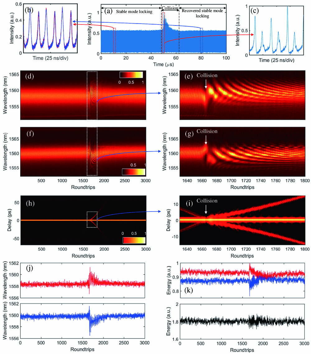
Fig. 2. Experimental real-time characterization of moderate collision of vector solitons. (a) Single-shot collision dynamics of vector solitons by the TS-DFT technique. (b), (c) Close-up of the data in (a) before, after, and during collision, respectively. (d), (f) Real-time spectral evolutions of the two vector solitons during collisions. (e), (g) Close-up of the data in (d), (f), respectively. (h) Field autocorrelation trace in (f) via Fourier transform. (i) Close-up of the data in (h). (j) Central wavelength evolutions of vector solitons (d), (f) during collisions. (k) Energies of both vector solitons (red and blue) and their total energy (black).
Fig. 3. Experimental real-time characterization of extreme collision of vector solitons. (a) Single-shot collision dynamics of vector solitons by the TS-DFT technique. (b) Close-up of the data in (a) after collision. (c), (e) Real-time spectral evolution of the two vector solitons during collisions. (d), (f) Close-up of the data in (c) and (e), respectively. (g) Field autocorrelation trace in (e) via Fourier transform. (h) Close-up of the data in (g).
Fig. 4. Numerical simulations of moderate collision of vector solitons. (a1), (b1), (e1) Spectral evolution, close-up of the data in (a1), and Kelly sideband rebuilding process of vector soliton in fast axis, respectively. (a2), (b2), (e2) Corresponding spectral evolution, close-up of the data in (a2), and Kelly sideband rebuilding process of vector soliton in slow axis, respectively. (c), (d), (f) Temporal evolution, field autocorrelation trace, and dispersive wave shedding of vector soliton in fast axis, respectively. (g1), (g2) Energy evolutions of vector solitons in fast (red) and slow (blue) axes, and total energy evolution. Inset: close-up of the data in (c).
Fig. 5. Numerical simulations of extreme collision of vector solitons. (a1), (a2) Spectral evolutions of the two vector solitons during collisions. (b1), (b2) Close-up of the data in (a1), (a2), respectively. (c1), (c2) Optical spectra at the 498th RT. (d1), (d2) Temporal traces at the 498th RT. (e1), (e2) Optical spectra of the dominant soliton [red curves, corresponding to the temporal traces in red boxes in (d)] and weak pulse [blue curves, corresponding to the temporal traces in blue boxes in (d)] by Fourier transform. (f1), (f2) Spectral evolutions of the dominant soliton and weak pulse, respectively, from the 490th to 500th RTs in (a2). Insets in (b2): close-up of the spectral evolutions (upper right) and temporal evolutions of the weak pulse (bottom right) from the 300th to 320th RTs.
Fig. 6. Numerical simulation results of (a), (b) total energy in each soliton and in each component, (c) temporal intensity, and (d) central wavelength in each soliton.


Set citation alerts for the article
Please enter your email address

© Copyright 2018-2021 | Chinese Laser Press. All Rights Reserved 沪ICP备15018463号-20