

Hai LI, Yang LI, Zheng-Rong ZUO. Detection of building area with complex background by night light remote sensing[J]. Journal of Infrared and Millimeter Waves, 2021, 40(3): 369
- Journal of Infrared and Millimeter Waves
- Vol. 40, Issue 3, 369 (2021)
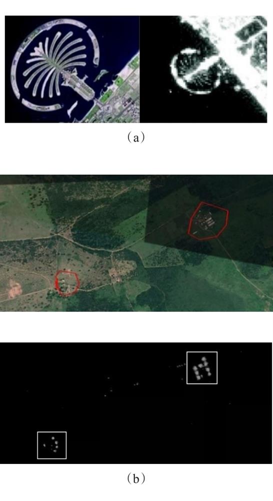
Fig. 1. Buildings are characterized by visible light remote sensing in night light remote sensing images(a) Local structural similarity(b) Remote context
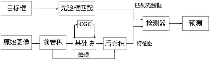
Fig. 2. Flow chart of detection network
Fig. 3. Four kinds of Classification network structure W
Fig. 4. Prior box matching correction
Fig. 5. 4 kinds of network detectors
Fig. 6. Sampling point graph of deformable convolution with unit number 9 passing through 3 layers
Fig. 7. Structure comparison between GC module and CGC module
Fig. 8. Two CGC connection modes
Fig. 9. RGB remote sensing picture and night light remote sensing picture(a) RGB of 123 object, (b)RGB of 4 object, (c) Sensing of 123 object, (d) Sensing of 4 object
Fig. 10. Sample picture of luminous remote sensing data set(object and category are marked in the picture)
Fig. 11. Network detection image(a)No module added(b)Add CGC2 module
Fig. 12. Different networks’ P-R curve
Fig. 13. Different networks’ F-measure
|
Table 1. Hidden layer characteristics of different networks
|
Table 2. Attention graphs of different global semantic modules
|
Table 3. All categories in the data set
|
Table 4. The performance of 4 kinds of networks on the night light remote sensing data set
|
Table 5. Adding expansion convolution in different stages
|
Table 6. Add GC module in different stages
|
Table 7. Comparison of ablation experiments of D-network modules
|
Table 8. Different network detection effects

Set citation alerts for the article
Please enter your email address
© Copyright 2018-2021 | Chinese Laser Press. All Rights Reserved 沪ICP备15018463号-20