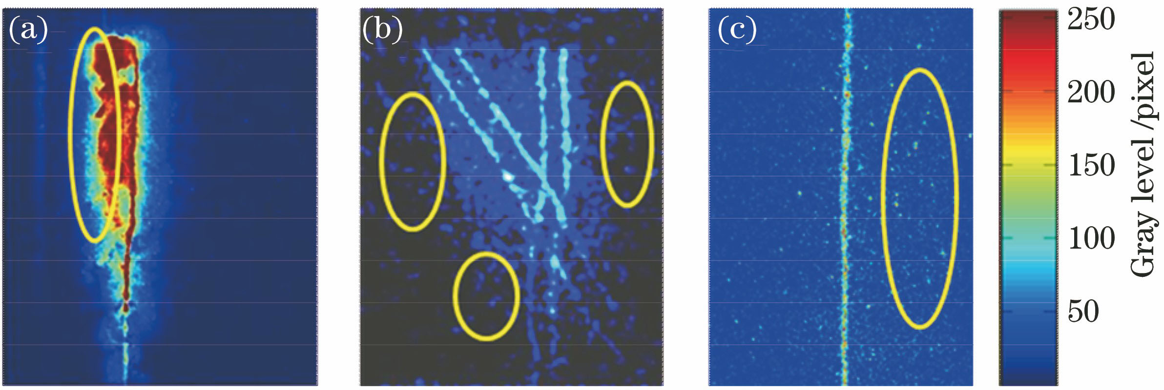
Fig. 1. HTV experimental images. (a) OHB fluorescence interference; (b) flow field noise; (c) system noise

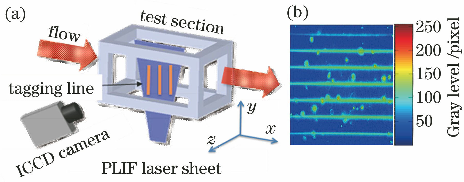
Fig. 2. Background noise. (a) Schematic of experimental setup; (b) experimental results

Fig. 3. Contrast of background noise in and out of PLIF display sheet

Fig. 4. Simulation images with background noise. (a) Simulation model with odd inflection points; (b) simulation model with even inflection points

Fig. 5. Background noise histogram image

Fig. 6. Standard deviation versus gain

Fig. 7. Contrast of simulation results and experimental results. (a) Simulation results; (b) experimental results

Fig. 8. Contrast of de-noising results of different parameters of simulation models. (a) Contrast of de-noising results with different window numbers with odd number of inflection points; (b) contrast of de-noising results with different window numbers with even number of inflection points; (c) evaluation of de-noising results of different signal models; (d) evaluation of de-noising results with different window sizes

Fig. 9. De-noising results of noise model. (a) Noise model; (b) ROI; (c) Hough detection; (d) partition filtering

Fig. 10. De-noising analysis of wavelet transform. (a)Model; (b)noised model; (c) RPSNR versus wavelet threshold coefficient; (d) RPSNR versus wavelet decomposition layer; (e) RPSNR versus wavelet iterated time; (f) RPSNR 、RSNR of de-noised signal versus RSNR of noised signal; (g) wavelet transform processing

Fig. 11. Flow diagram of image preprocessing

Fig. 12. Contrast of simulation de-noising results. (a) Noised model; (b) Gaussian smoothing; (c) median filtering; (d) Laplace sharpening; (e) spatial filtering; (f) proposed method

Fig. 13. Experimental locale photo

Fig. 14. De-noising results of experimental data. (a) Experimental image; (b) proposed method result; (c) Gaussian smoothing result; (d) median filtering result; (e) Laplace sharpening result

Table 1. Characteristic analysis of background noise

Table 2. Background noise processing methods

Table 3. Contrast of de-noising results