• Photonics Research
  • Vol. 9, Issue 11, 2261 (2021)
Qian Cao1, Jian Chen1, Keyin Lu1, Chenhao Wan1、2, Andy Chong3、4, and Qiwen Zhan1、*
Author Affiliations
  • 1School of Optical-Electrical and Computer Engineering, University of Shanghai for Science and Technology, Shanghai 200093, China
  • 2School of Optical and Electronic Information, Huazhong University of Science and Technology, Wuhan 430074, China
  • 3Department of Physics, University of Dayton, Dayton, Ohio 45469, USA
  • 4Department of Electro-Optics and Photonics, University of Dayton, Dayton, Ohio 45469, USA
  • show less
    DOI: 10.1364/PRJ.439849 Cite this Article Set citation alerts
    Qian Cao, Jian Chen, Keyin Lu, Chenhao Wan, Andy Chong, Qiwen Zhan. Sculpturing spatiotemporal wavepackets with chirped pulses[J]. Photonics Research, 2021, 9(11): 2261 Copy Citation Text show less
    Schematic of STWP generator and 3D wavepacket characterization. The experimental setup for generating and characterizing STWP. The upper arm is an STWP generator, which applies an x-ω phase to an input wavepacket. A positively chirped Gaussian–Gaussian wavepacket is modulated by a two-dimensional phase on the x-ω plane and transformed into the desired wavepacket. A helical phase pattern is used as an example for the generation of STOV. The tilt of the pulse is used to illustrate different arrival times for different frequency components. The lower arm of the setup is a reference arm that delivers a compressed probe pulse to characterize the generated STWP from the upper arm. Two wavepackets overlap on the CCD with an incident angle offset of θ. By scanning their relative time delay, 3D intensity and phase profiles of the STWP can be retrieved [9].
    Fig. 1. Schematic of STWP generator and 3D wavepacket characterization. The experimental setup for generating and characterizing STWP. The upper arm is an STWP generator, which applies an x-ω phase to an input wavepacket. A positively chirped Gaussian–Gaussian wavepacket is modulated by a two-dimensional phase on the x-ω plane and transformed into the desired wavepacket. A helical phase pattern is used as an example for the generation of STOV. The tilt of the pulse is used to illustrate different arrival times for different frequency components. The lower arm of the setup is a reference arm that delivers a compressed probe pulse to characterize the generated STWP from the upper arm. Two wavepackets overlap on the CCD with an incident angle offset of θ. By scanning their relative time delay, 3D intensity and phase profiles of the STWP can be retrieved [9].
    ST intensity of STOV wavepackets with different amounts of GDD. The STOV wavepacket is characterized at 85 cm after the STWP generator. With different amounts of GDD added, STOV wavepackets exhibit different ST intensity profiles. The wavepacket has a ring-like intensity pattern when GDD is positive. When STOV wavepacket has a negative GDD, the ST intensity profile is distorted because of the astigmatism between dispersion and diffraction. (a), (c), (e) STOV wavepackets with a charge of l=+1. (b), (d), (f) STOV wavepackets with a charge of l=+2.
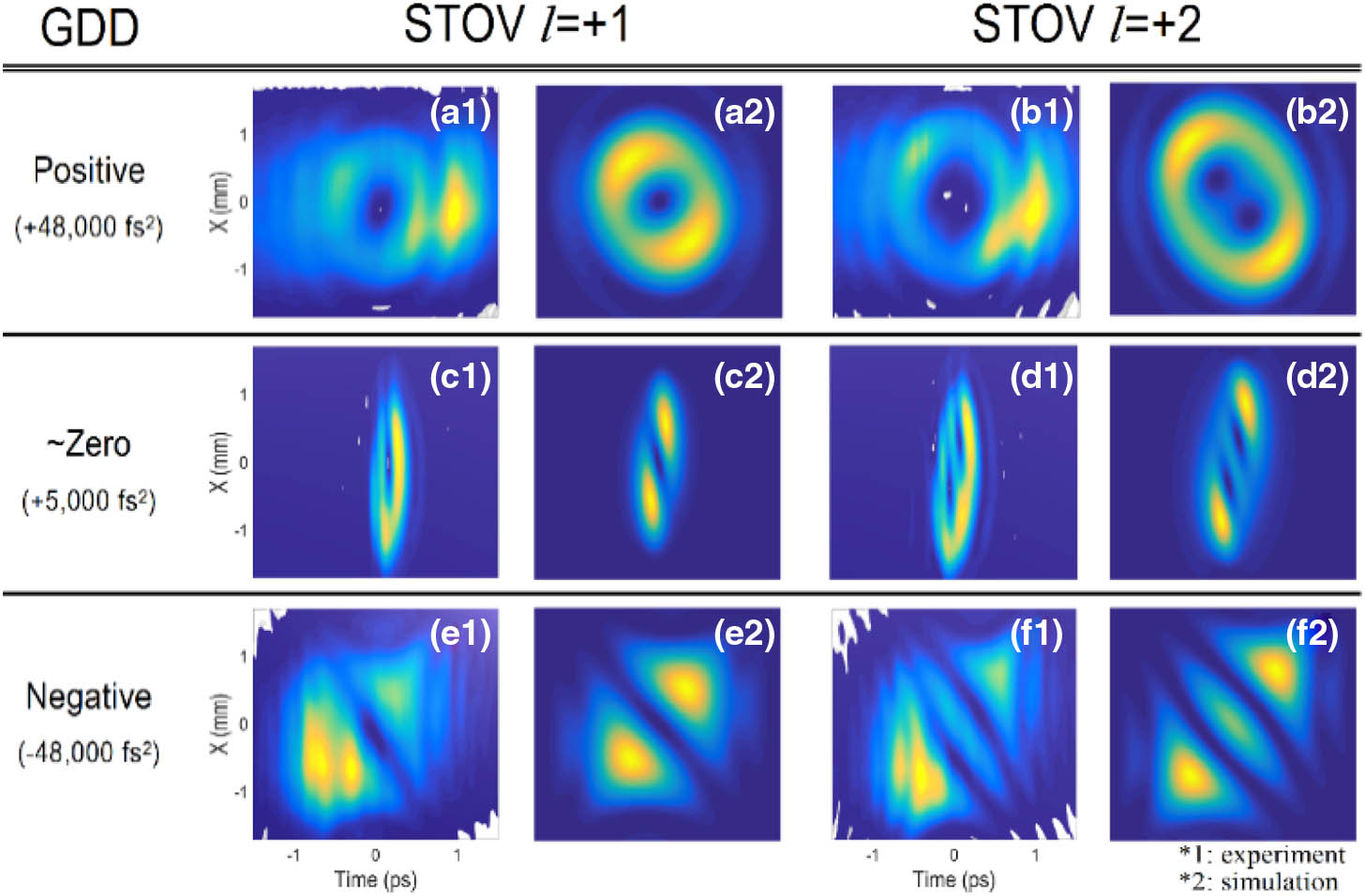
    Fig. 2. ST intensity of STOV wavepackets with different amounts of GDD. The STOV wavepacket is characterized at 85 cm after the STWP generator. With different amounts of GDD added, STOV wavepackets exhibit different ST intensity profiles. The wavepacket has a ring-like intensity pattern when GDD is positive. When STOV wavepacket has a negative GDD, the ST intensity profile is distorted because of the astigmatism between dispersion and diffraction. (a), (c), (e) STOV wavepackets with a charge of l=+1. (b), (d), (f) STOV wavepackets with a charge of l=+2.
    ST phase profile of STOV wavepackets with different amounts of GDD. ST phase is measured for the STOV wavepackets with different GDD. The ST phase has a topological charge with opposite sign when different GDD is imposed to the wavepacket. When overall GDD is positive, the STOV charge aligns with the added ST spiral phase. Conversely, when overall GDD is negative, the STOV charge has a reversed sign. (a), (c) STOV wavepackets with an applied STOV charge of l=+1. (b), (d) STOV wavepackets with an applied STOV charge of l=+2.
    Fig. 3. ST phase profile of STOV wavepackets with different amounts of GDD. ST phase is measured for the STOV wavepackets with different GDD. The ST phase has a topological charge with opposite sign when different GDD is imposed to the wavepacket. When overall GDD is positive, the STOV charge aligns with the added ST spiral phase. Conversely, when overall GDD is negative, the STOV charge has a reversed sign. (a), (c) STOV wavepackets with an applied STOV charge of l=+1. (b), (d) STOV wavepackets with an applied STOV charge of l=+2.
    STOV lattice with multiple STOVs multiplexed in space and time. (a) Four elemental (l=+1) STOV wavepackets in space and time. (b) Four elemental STOV wavepackets with alternating STOV polarity. (c) Four STOV wavepackets with different STOV charge (l1=−1, l2=+2, l3=l4=+1). (d)–(f) Corresponding measured ST phase profiles of spatiotemporally multiplexed STOV wavepackets.
    Fig. 4. STOV lattice with multiple STOVs multiplexed in space and time. (a) Four elemental (l=+1) STOV wavepackets in space and time. (b) Four elemental STOV wavepackets with alternating STOV polarity. (c) Four STOV wavepackets with different STOV charge (l1=1, l2=+2, l3=l4=+1). (d)–(f) Corresponding measured ST phase profiles of spatiotemporally multiplexed STOV wavepackets.
    ST collision of two STOVs. Linear phases with opposite signs are applied on the left/right side of the input light field to advance/delay input wavepackets in the corresponding time domain. The phase is expressed as ϕ(ω)=kt|ω−ω0|. Subplots (a)–(e) show the collision of two STOVs with same STOV charge l1=l2=+1. From (a1) to (e1), the linear phase coefficient kt changes from −450 fs to +450 fs. Subplots (f)–(j) show the collision of two STOVs with different STOV charges l1=+1 and l2=−1.
    Fig. 5. ST collision of two STOVs. Linear phases with opposite signs are applied on the left/right side of the input light field to advance/delay input wavepackets in the corresponding time domain. The phase is expressed as ϕ(ω)=kt|ωω0|. Subplots (a)–(e) show the collision of two STOVs with same STOV charge l1=l2=+1. From (a1) to (e1), the linear phase coefficient kt changes from 450  fs to +450  fs. Subplots (f)–(j) show the collision of two STOVs with different STOV charges l1=+1 and l2=1.
    Qian Cao, Jian Chen, Keyin Lu, Chenhao Wan, Andy Chong, Qiwen Zhan. Sculpturing spatiotemporal wavepackets with chirped pulses[J]. Photonics Research, 2021, 9(11): 2261
    Download Citation