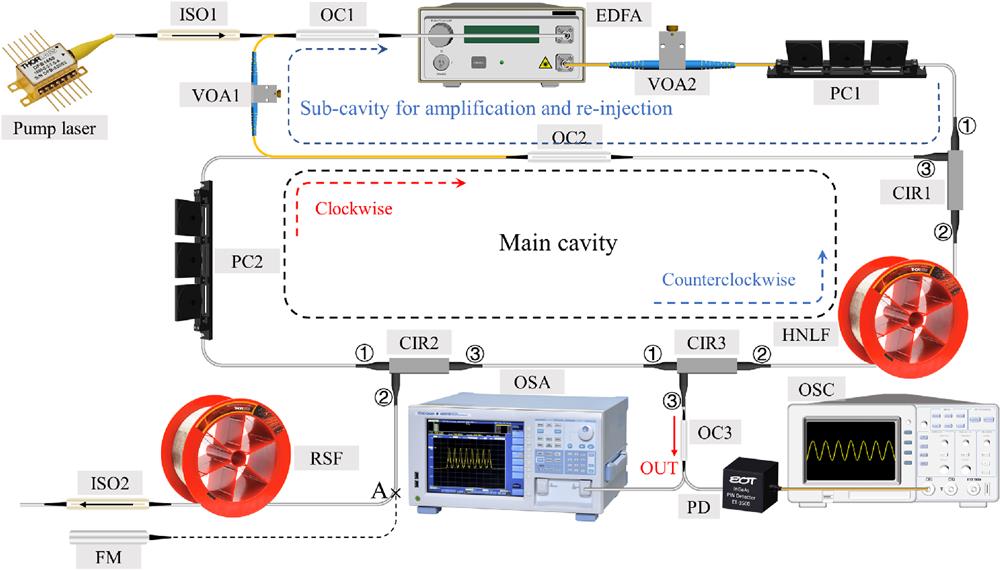
Fig. 1. Experimental setup of the BRFLC. (ISO, isolator; OC, optical coupler; EDFA, erbium-doped fiber amplifier; VOA, variable optical attenuator; PC, polarization controller; CIR, circulator; HNLF, highly nonlinear fiber; RSF: Rayleigh scattering fiber; OSA, optical spectrum analyzer; PD, photodetector; OSC, oscilloscope; FM, fiber mirror.

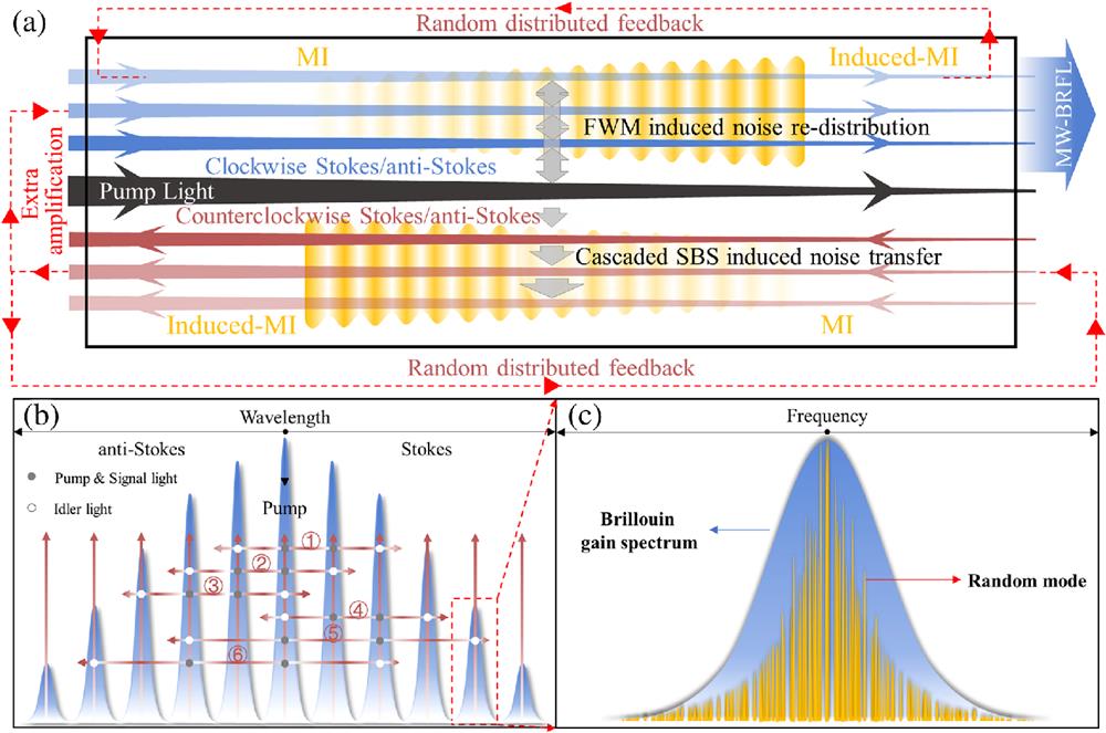
Fig. 2. Schematic diagram of (a) the operation principle of the BRFLC and the interplay among the noise-driven MI, the cascaded SBS, and the quasi-phase-matched FWM process; (b) the cascaded SBS process and the quasi-phase-matched FWM process occurring among multiple Stokes and anti-Stokes lines; and (c) random mode distribution within the Brillouin gain spectrum for a certain Stokes/anti-Stokes line.

Fig. 3. Simulations of parametric gain coefficient versus (a) linear phase shift Δβ and (b) order-difference up to 60 for both Stokes and anti-Stokes lights at different sum powers of 50, 100, 150, and 200 mW of two interacting Stokes/anti-Stokes lights as the pump and signal lights in the quasi-phase-matched FWM process.

Fig. 4. Measured optical spectrum of the BRFLC output (a) at different pump powers and (b) at a pump power of 810 mW with 21 orders of Stokes lights and 18 orders of anti-Stokes lights; power spectra of the first-order Stokes lights of the Brillouin fiber laser comb with (c) random distributed feedback and (d) mirror feedback.

Fig. 5. Statistical histograms (left panel) of the pulse amplitudes in typical temporal traces (right panel) of first- to eighth-order (a) Stokes and (b) anti-Stokes lights at the pump power of 810 mW. The red dashed lines mark the 2×SWH.

Fig. 6. Evolution of the proportion of optical RWs as a function of (a) the Stokes and (b) anti-Stokes order, and as a function of pump power for (c) Stokes and (d) anti-Stokes lights of different orders; evolution of the proportion of optical RWs as a function of (e) Stokes and (f) anti-Stokes order for cases of random distributed feedback provided by RSFs of different lengths and mirror feedback (green line), respectively.

Fig. 7. (a) Temporal trace of the fourth-order Stokes light in a time span of 5 ms; (b) close-up view of the temporal trace in a time span of 6μs; (c) evolution of consecutive temporal traces around temporally localized optical RW events of the second-order Stokes light at a pump power of 810 mW; inset, typical pulse shapes of the RW1 and RW2. The black dashed lines mark the 2×SWH.

Fig. 8. Statistical histograms of output amplitude of (a) the first-order Stokes, (b) second-order Stokes, (c) third-order Stokes, (d) fourth-order Stokes, (e) first-order anti-Stokes, and (f) second-order anti-Stokes lights with linear (blue) and logarithmic (red) count scale. The red and black dashed vertical lines mark the 2×SWH and the amplitude of the counting peak, respectively.

Fig. 9. Temporal traces, typical pulse shape, and statistical distribution of duration of chair-like pulses in the output of (a) first-order Stokes, (b) second-order Stokes, (c) third-order Stokes, (d) fourth-order Stokes, (e) first-order anti-Stokes, and (f) second-order anti-Stokes lights at a pump power of 810 mW. The red and black dashed lines mark the amplitude of the trailing plateau of the chair-like pulse and the 2×SWH, respectively.

Fig. 10. Pulse shapes of the temporally localized optical RWs appearing in (a1–a5) the first-order Stokes, (b1–b5) second-order Stokes, (c1–c5) third-order Stokes, (d1–d5) sixth-order Stokes, and (e1–e5) second-order anti-Stokes lights. The black and red dashed lines mark the 2×SWH and the amplitude of the trailing plateau of the chair-like pulse, respectively.

Fig. 11. Duration manipulation for temporally localized optical RWs in (a1–a9) the first-order Stokes, (b1–b7) second-order Stokes, (c1–c6) third-order Stokes, and (d1–d6) fourth-order Stokes lights realized by adjusting the pumping power. The black and red dashed lines mark the 2×SWH and the amplitude of the trailing plateau of the chair-like pulse, respectively.