
Xin He, Jian Zhou, Xiaoming Nie, Xingwu Long. Filtering characteristics of spatial filter for spatial filtering velocimeter[J]. Chinese Optics Letters, 2015, 13(6): 060702
- Chinese Optics Letters
- Vol. 13, Issue 6, 060702 (2015)
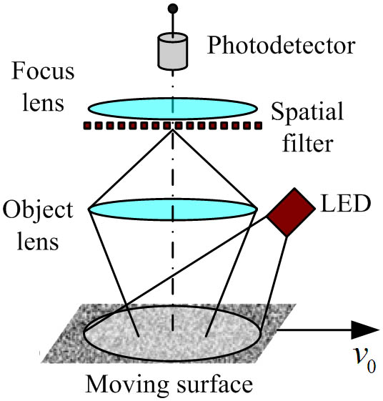
Fig. 1. Basic setup of a spatial filtering velocimeter.
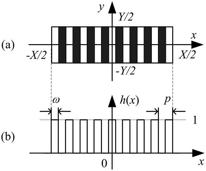
Fig. 2. Schematic diagram of (a) a rectangular-type spatial filter with rectangular transmittance and (b) its transmittance function.
Fig. 3. Power spectrum of a rectangular-type spatial filter with rectangular transmittance for n = 10
Fig. 4. Schematic diagram of (a) a rectangular-type differential spatial filter with rectangular transmittance and (b) its transmittance function.
Fig. 5. Power spectrum of a rectangular-type differential spatial filter with rectangular transmittance for n = 10
Fig. 6. Power spectra H p ( f x , 0 ) n = 2
Fig. 7. Power spectra H p ( f x , 0 ) n = 2
Fig. 8. Dependence of the specific bandwidth on the number of spatial periods n
Fig. 9. Influence of pedestal components f x p = 0 f x = 1 / p
Fig. 10. Influence of higher spatial frequencies on the deviation of the central frequency f x = 1 / p f x p = 1
Fig. 11. Interaction of f x p = 1 f x p = − 1 f x = 1 / p f x p = 1 f x p = − 1
Fig. 12. Dependence of the peak value of transmittance on the number of spatial periods n
| ||||||||||||||||||||||||||||||||||||||||||||||||||||||||||||||||||||
Table 1. Dependence and Quantization of the Deviation ε on the Number of Spatial Periods n for Both Common and Differential Filters

Set citation alerts for the article
Please enter your email address
© Copyright 2018-2021 | Chinese Laser Press. All Rights Reserved 沪ICP备15018463号-20