Filtering characteristics of spatial filter for spatial filtering velocimeter

Xin He; Jian Zhou; Xiaoming Nie; Xingwu Long

doi:10.3788/COL201513.060702

Abstract

In order to select a suitable spatial filter for the spatial filtering velocimeter, the filtering characteristics of the spatial filters with a rectangular window and rectangular transmittance are investigated by the power spectrum of transmittance function method. The filtering characteristics of differential filters are investigated and compared with that of common ones. The influences of the number of spatial periods on the spectral bandwidth, deviation to central frequency, and peak transmittance are deeply analyzed. The results show that the influence is due to the form of superposition of the signal components and other components, the pedestal and higher-order components, and the superposition results from the finite size of the spatial filter. According to the results, a method is proposed to compensate for the deviation to central frequency.

Since it was proposed in about the 1960s by Ator^[1], much attention has been paid to spatial filtering velocimetry (SFV) because of its simplicity and the stability of the optical and mechanical system. The main research interest in SFV has been focused on the design of the spatial filter. In SFV, periodic output signals carrying velocity information are produced by the narrow-band frequency component selected at $f_{x} p = \pm 1$ in the power spectrum of the spatial filter’s transmittance function^[2], where $f_{x}$ is the spatial frequency and $p$ is the spatial period of the spatial filter. Thus, the signal quality primarily depends on the filtering characteristics of the narrow-bandpass peak in the power spectrum.

The spatial filters mainly have three kinds of windows: rectangular, circular, and Gaussian. Each window has several transmittance functions, for example, sinusoidal and rectangular transmittance functions. Filtering characteristics of spatial filters with a circular window and sinusoidal transmission have been analyzed^[2]. In recent years, image sensors or cameras have been widely applied^[3–6], and the use of an image sensor both as a spatial filter and a photodetector has been introduced to SFV^[6–10]. The image-type spatial filter has a rectangular window and a rectangular transmittance function if no weighting function is applied. Spatial filters with a rectangular transmission are much more complicated than filters with a sinusoidal transmission since they have higher orders of spatial frequency. Here we investigate the spatial filtering characteristics, the spectral bandwidth, the central frequency of the periodic signal component, and the peak value of the transmittance in the power spectra of spatial filters having a rectangular window and a rectangular transmittance function.

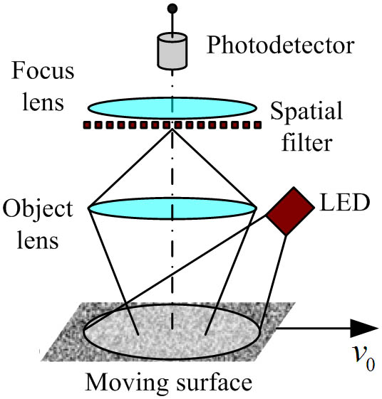
Figure 1 shows the basic setup of a spatial filtering velocimeter. A white light source is employed as the active illumination. The illuminated measured moving surface is imaged onto the spatial filter by an object lens. The variation of the total intensity of surface image passes through the spatial filter and is focused into a photodetector, where it is converted to a temporal signal containing a frequency $f$ proportional to the object velocity $v$ . This relationship can be given as $v = p f / M,$ (1)where $p$ is the spatial period of the spatial filter and $M$ is the magnification of the imaging system.

Sign up for Chinese Optics Letters TOC. Get the latest issue of Chinese Optics Letters delivered right to you！Sign up now

Figure 1.Basic setup of a spatial filtering velocimeter.

A basic spatial filter is a set of parallel slits. Figure 2 shows the schematic diagram of a rectangular-type spatial filter with a rectangular transmittance and its transmittance function. It is assumed that the filter has a size of $X$ in the $x$ direction, and a size of $Y$ in the $y$ direction. Then the transmittance function can be given by $h (x, y) = {\begin{matrix} 1, & (l p - \frac{ω}{2}) \leq x \leq (l p + \frac{ω}{2}), - \frac{X}{2} \leq x \leq \frac{X}{2}, - \frac{Y}{2} \leq y \leq \frac{Y}{2}, \\ 0, & otherwise . \end{matrix}$ (2)where $l$ is an integer, $ω$ is the width of the slits, and $p$ is the space of two neighboring slits. If $p = 2 ω$ , the power spectrum of $h (x, y)$ can be deduced as^[2] $H_{p} (f_{x}, f_{y}) = \frac{X^{2} Y^{2}}{4} {| H_{Y} (f_{y}) |}^{2} {[H_{X} (f_{x}) + H_{X m} (f_{x})]}^{2},$ (3) $H_{Y} (f_{y}) = \sin c (f_{y} Y),$ (4) $H_{X} (f_{x}) = \sin c (f_{x} X),$ (5) $H_{X m} (f_{x}) = \sum_{m = 1}^{\infty} {(- 1)}^{m - 1} \frac{2}{(2 m - 1) π} [H_{X m}^{-} (f_{x}) + H_{X m}^{+} (f_{x})],$ (6) $H_{X m}^{-} (f_{x}) = \sin c (f_{x} X - \frac{2 m - 1}{p} X),$ (7) $H_{X m}^{+} (f_{x}) = \sin c (f_{x} X + \frac{2 m - 1}{p} X),$ (8)where $f_{x}$ and $f_{y}$ denote the spatial frequencies in the $x$ and $y$ directions, respectively. Equations (7) and (8) can be written as $H_{X m}^{-} (f_{x}) = \sin c {[f_{x} p - (2 m - 1)] n},$ (9) $H_{X m}^{+} (f_{x}) = \sin c {[f_{x} p + (2 m - 1)] n},$ (10)where $n = X / p$ is the number of spatial periods. Figure 3 shows the power spectrum of a rectangular-type spatial filter with rectangular transmittance for $n = 10$ . Figure 3 has peaks at $f_{x} p = \pm (2 m - 1)$ , but only the peaks at $f_{x} p = \pm 1$ are used to detect velocities. That is to say, the spatial filter selects the spatial frequency $f_{x} = 1 / p$ . The peak at $f_{x} p = 0$ , called the pedestal, resulting from Eq. (5), is not useful and should be eliminated.

Figure 2.Schematic diagram of (a) a rectangular-type spatial filter with rectangular transmittance and (b) its transmittance function.

Figure 3.Power spectrum of a rectangular-type spatial filter with rectangular transmittance for $n = 10$ .

Generally, a differential spatial filter is used to eliminate $f_{x} p = 0$ . Figure 4 shows the schematic diagram of a rectangular-type differential spatial filter with a rectangular transmittance and its transmittance function. The transmittance function can be given by $h (x, y) = {\begin{cases} 1, & (l p - \frac{ω}{2}) \leq x \leq (l p + \frac{ω}{2}), - \frac{X}{2} \leq x \leq \frac{X}{2}, - \frac{Y}{2} \leq y \leq \frac{Y}{2}, \\ - 1, & (l p + \frac{ω}{2}) \leq x \leq (l p + \frac{3 ω}{2}), - \frac{X}{2} \leq x \leq \frac{X}{2}, - \frac{Y}{2} \leq y \leq \frac{Y}{2}, \\ 0, & otherwise . \end{cases}$ (11)

Figure 4.Schematic diagram of (a) a rectangular-type differential spatial filter with rectangular transmittance and (b) its transmittance function.

This type of differential filter can be constructed by an image sensor^[11,12]. If $p = 2 ω$ , the power spectrum of $h (x, y)$ can be deduced as $H_{p} (f_{x}, f_{y}) = \frac{X^{2} Y^{2}}{4} {| H_{Y} (f_{y}) |}^{2} {[H_{X m} (f_{x})]}^{2},$ (12) $H_{X m} (f_{x}) = \sum_{m = 1}^{\infty} {(- 1)}^{m - 1} \frac{4}{(2 m - 1) π} [H_{X m}^{-} (f_{x}) + H_{X m}^{+} (f_{x})] .$ (13)

A comparison of Eqs. (3) and (12) indicates that the pedestal components are eliminated by a differential method. Figure 5 shows the power spectrum of a rectangular type of differential spatial filter with a rectangular transmittance for $n = 10$ .

Figure 5.Power spectrum of a rectangular-type differential spatial filter with rectangular transmittance for $n = 10$ .

In both Figs. 3 and 5, the number of spatial periods is specified as $n = 10$ since it has great impact on power spectra. Figures 6 and 7 show, respectively, power spectra for common and differential rectangular-type and rectangular-transmission spatial filters with different spatial periods $n$ . It can be seen that the peaks around $f_{x} p = \pm 1$ are broadened and deviate from $f_{x} p = \pm 1$ , which limits the basic accuracy for measurements of the central frequency in output signals. With increasing $n$ , the bandwidth becomes narrower and the deviation becomes less significant. For the same value of $n$ , the bandwidths in the two figures are about the same. However, the peaks in Fig. 7 deviate less compared with that in Fig. 6. This means that a differential filter can reduce the deviation of the spatial frequency as well as quadruple the peak transmittance. Here we investigate the bandwidth and the deviation of the central frequency for both common and differential spatial filters and propose a method to eliminate the influence of the deviation of the central frequency. The dependence of the peak transmittance on the number of spatial periods $n$ for common and differential filters is also discussed.

Figure 6.Power spectra $H_{p} (f_{x}, 0)$ for a rectangular-type rectangular-transmission spatial filter with $n = 2$ , 4, 8, and 16.

Figure 7.Power spectra $H_{p} (f_{x}, 0)$ for a differential rectangular-type rectangular-transmission spatial filter with $n = 2$ , 4, 8, and 16.

To evaluate the spectral bandwidth, a parameter $D$ is introduced as the bandwidth of the peak spectrum normalized by the fundamental spatial frequency and is called the specific bandwidth. In the power spectrum with $f_{x} p$ as the $x$ coordinate, $D$ is the half-value full width of the peak at $f_{x} p = \pm 1$ . As seen from Figs. 6 and 7, $D$ is decreasing with increasing $n$ . Figure 8 illustrates the dependence of the specific bandwidth on the number of spatial periods $n$ for both common and differential spatial filters. The specific bandwidths of the two kinds of filters show no significant difference. The relationship between $n$ and $D$ in a differential filter is fitted as $D = \frac{0.8924}{n} .$ (14)

Figure 8.Dependence of the specific bandwidth on the number of spatial periods $n$ for both common and differential filters.

Equation (14) shows that $n$ and $D$ have an inversely proportional relationship. Spectral broadening degrades the selectivity of the spatial filter and limits the basic accuracy for measurements of the central frequency in output signals. In addition, under the condition of small $n$ and lower spatial frequency, spectral broadening makes the peaks $f_{x} p = 0$ and $f_{x} p = \pm 1$ overlap significantly, making it difficult to detect low frequencies. Thus, a large number of $n$ is desired, generally.

As shown in Figs. 6 and 7, the peaks deviate from $f_{x} p = \pm 1$ , which means the deviation results from both the pedestal components and the other orders of spatial frequencies. Let us first discuss how the pedestal components influence the deviation. Figure 9 shows the influence of pedestal components $f_{x} p = 0$ on the deviation of the central frequency $f_{x} = 1 / p$ for $n = 2$ , 3, 4, and 5, respectively. The signal component $f_{x} p = 1$ (shown by the red curve) is calculated and plotted separately from the pedestal components $f_{x} p = 0$ (shown by the green curve), and the two of them are calculated and plotted together (shown by the blue curve). The red curve shows that the central frequency does not deviate from $f_{x} = 1 / p$ at all. However, because of the influence of the tails of the pedestal components, it deviates to a higher frequency for $n = 2$ and 4, to a lower frequency for $n = 3$ and 5. The tails of the pedestal components gradually attenuate and the influence becomes less significant with increasing $n$ .

Figure 9.Influence of pedestal components $f_{x} p = 0$ on the deviation of the central frequency $f_{x} = 1 / p$ . The signal (red curve) and pedestal components (green curve) are separately calculated and plotted. The two of them are plotted together by the blue curve.

Figure 10 shows the influence of higher orders of spatial frequencies ( $| f_{x} p | = 3,5, 7, \dots$ ) on the deviation of the central frequency $f_{x} = 1 / p$ for $n = 2$ and 4, respectively. The signal component $f_{x} p = 1$ (shown by the red curve) is calculated and plotted separately from these higher orders of spatial frequencies $| f_{x} p | = 3,5, 7, \dots$ (shown by the green curve), and the two of them are calculated and plotted together (shown by the blue curve). The red curve shows that the central frequency does not deviate from $f_{x} = 1 / p$ at all. However, because of the influence of the tails of the higher orders of spatial frequencies, it deviates to a higher frequency. The tails of the higher spatial frequencies gradually attenuate and the influence becomes less significant with increasing $n$ .

Figure 10.Influence of higher spatial frequencies on the deviation of the central frequency $f_{x} = 1 / p$ . The signal $f_{x} p = 1$ (red curve) and higher spatial frequencies (green curve) are separately calculated and plotted. The two of them are plotted together by the blue curve.

In fact, the peaks of $f_{x} p = \pm 1$ themselves have interactions. Figure 11 shows the interaction of $f_{x} p = 1$ and $f_{x} p = - 1$ on the deviation of central frequency $f_{x} = 1 / p$ . The signal components $f_{x} p = 1$ (shown by the red curve) and $f_{x} p = - 1$ (shown by the green curve) are calculated and plotted separately, and the two of them are calculated and plotted together (shown by the blue curve). The red curve and green curve show the central frequency does not deviate from $f_{x} = \pm 1 / p$ at all. However, because of the tails of $f_{x} p = - 1$ ( $f_{x} p = 1$ ), the central frequency deviates from $f_{x} = 1 / p$ ( $f_{x} = - 1 / p$ ). The tails of the two peaks gradually attenuate and the influence becomes less significant with increasing $n$ .

Figure 11.Interaction of $f_{x} p = 1$ and $f_{x} p = - 1$ on the deviation of central frequency $f_{x} = 1 / p$ . $f_{x} p = 1$ (red curve) and $f_{x} p = - 1$ (green curve) are separately calculated and plotted. The two of them are plotted together by the blue curve.

To sum up, because of the influences of the three factors discussed above, namely the pedestal components $f_{x} p = 0$ , higher orders of spatial frequencies, and the interaction of $f_{x} p = \pm 1$ themselves, the selected spatial frequency $f_{x}$ deviates from $1 / p$ , resulting in $f_{x} p > 1$ or $f_{x} p < 1$ . However, in Eq. (1) $f_{x} p = 1$ is used. Therefore, the use of Eq. (1) to calculate velocities will introduce inaccuracy.

To evaluate the deviation of the central frequency, a deviation is defined by the peak deviation $Δ (f_{x} p)$ from $f_{x} p = 1$ as $ε = Δ (f_{x} p) .$ (15)

Table 1 shows the dependence and quantization of the deviation $ε$ on the number of spatial periods $n$ for both common and differential filters. In both of the two filters, the deviation is decreasing with increasing $n$ . However, deviation $ε$ in differential filters is always above zero, while in common filters the central frequency deviates to a lower frequency and higher frequency, alternatively. It seems that the pedestal components have a more significant influence on filters having an even number of spatial periods than on filters having an odd number of spatial periods. In differential spatial filters, for $n \geq 14$ , the deviation from the central frequency is less than 0.1%. Therefore, for accurate measurement applications, it is recommended that $n \geq 14$ in differential filters.

	Deviation of central frequency
n	Common filter/ε1	Differential filter/ε2	ε1/ε2
2	0.1100	0.0410	2.68
3	−0.0358	0.0190	−1.88
4	0.0354	0.0110	3.22
5	−0.0125	0.0070	−1.79
6	0.0170	0.0054	3.15
7	−0.0063	0.0030	−2.10
8	0.0100	0.0027	3.70
9	−0.0037	0.0021	−1.76
10	0.0060	0.0017	3.53
11	−0.0025	0.0014	−1.79
12	0.0040	0.0012	3.33
13	−0.0017	0.0010	−1.70
14	0.0030	0.0009	3.33
15	−0.0012	0.0008	−1.50
16	0.0020	0.0007	2.86

Table 1. Dependence and Quantization of the Deviation ε on the Number of Spatial Periods n for Both Common and Differential Filters

View all Tables

However, for common filters or for differential filters when $n \leq 13$ , Eq. (1) must be corrected to eliminate inaccuracy introduced by the deviation of the central frequency, as $v = \frac{1}{(1 + ε)} p f / M,$ (16)where $ε$ can be looked up in Table 1.

As shown in Figs. 6 and 7, the peak transmittance of $f_{x} = 1 / p$ varies in both common and differential spatial filters. Consequently, the dependence of the peak value of transmittance on the number of spatial periods $n$ for both common and differential filters is investigated, and the result is shown in Fig. 12. In common filters, the peak value decreases with fluctuation, with increasing $n$ ; the difference of peak transmittance for small and large $n$ is as big as 25%. This mainly results from the tails of the pedestal components since the tails overlap the signal components. In differential filters, the peak value decreases without fluctuation, with increasing $n$ , and the difference of the peak transmittance for small and large $n$ becomes very small. This mainly results from the tails of higher orders of spatial frequency since the tails overlap the signal components and the influence of these higher orders is insignificant compared with that of the pedestal. As discussed above, the comparison of Eqs. (6) and (13) indicates that the coefficients are doubled, so the coefficients in Eq. (12) for differential filters are four times that of common ones. However, in Fig. 12, for small numbers of $n$ , the peak transmittance in differential filters is about three times that of common ones, while for large numbers of $n$ , the multiple is about four. This difference is caused by the tails of the pedestal components since for small $n$ the influence of the tails is significant.

Figure 12.Dependence of the peak value of transmittance on the number of spatial periods $n$ for (a) common and (b) differential filters.

In conclusion, the spatial filtering characteristics of the spatial filters with a rectangular window and a rectangular transmittance in SFV are analyzed theoretically. By comparison of the analysis results of common and differential filters it is found that in common filters the transmittance of the signal frequency is mostly influenced by the pedestal components, while in differential ones it is influenced by higher orders of spatial frequency and the signal components themselves. The pedestal components are more influential than other orders of spatial frequency. The filtering characteristics, bandwidth broadening, deviation from central frequency, and variation of peak value of transmittance result from the finite size of the spatial filters or finite number of spatial period. The finite size makes every order of spatial frequency have tails that overlap each other. These tails gradually attenuate with increasing $n$ , and the overlap becomes less significant. Therefore, a big number of spatial period leads to a narrow bandwidth, small deviation to a central frequency and a small peak transmittance. In practical use, a big $n$ is recommended. What is more, the deviation to a central frequency is quantized and a correction to the equation $v = p f / M$ is proposed to eliminate the deviation, making the measurement more accurate.

References

[1] J. T. Ator. J. Opt. Soc. Am., 53, 1416(1963).

[2] Y. Aizu, T. Asakura. Spatial Filtering Velocimetry: Fundamentals and Applications(2005).

[3] H. Ye, Z. Gao, Z. Qin, Q. Wang. Chin. Opt. Lett., 11, 31702(2013).

[4] Y. Yan, L. Wei, X. Wen, Y. Wu, Z. Zhao, B. Zhang, B. Zhu, W. Hong, L. Cao, Z. Yao, Y. Gu. Chin. Opt. Lett., 11, 110401(2013).

[5] Y. Wang, F. Zhou, Y. Cui. Chin. Opt. Lett., 12, 101301(2014).

[6] X. He, J. Zhou, X. Nie, X. Long. Opt. Eng., 54, 34110(2015).

[7] K. C. Michel, O. F. Fiedler, A. Richter, K. Christofori, S. Bergeler. IEEE Trans. Instrum. Meas., 47, 299(1998).

[8] Z. Dong, K. Michel, S. Bergeler, K. Christofori, H. Krambeer. Chin. J. Sci. Instrum., 21, 211(2000).

[9] S. Bergeler, H. Krambeer. Meas. Sci. Technol., 15, 1309(2004).

[10] X. He, X. Nie, J. Zhou, X. Long. Optik, 125, 7136(2014).

[11] L. Zheng, H. Kuang, W. Li, X. Leng, G. Yuan, X. Chen. Acta Opt. Sin., 34, 211001(2014).

[12] H. Xin, L. Xingwu, Z. Jian, N. Xiaoming. Acta Opt. Sin., 35, 0512006(2015).