
Chunping Hou, Kaixin Cao, Zhipeng Wang. Environment Pre-Judgment Model of Substation Meter Reading[J]. Laser & Optoelectronics Progress, 2021, 58(12): 1210026
- Laser & Optoelectronics Progress
- Vol. 58, Issue 12, 1210026 (2021)
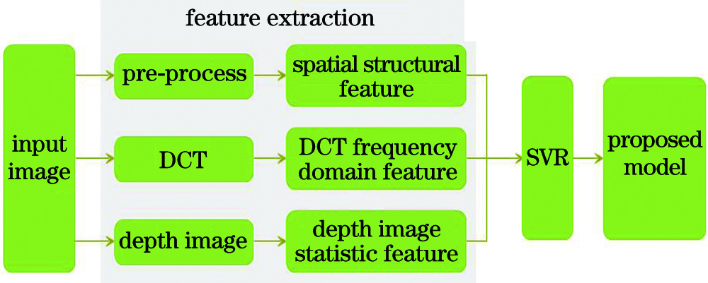
Fig. 1. Framework of environmental prejudgment model for meter reading
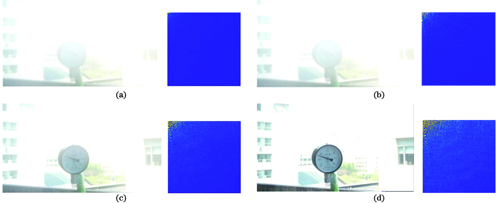
Fig. 2. Meter images and DCT transform images under different fog concentrations. (a) Images with score of 1; (b) images with score of 3; (c) images with score of 5; (d) images with score of 7
Fig. 3. Meter images and LBP images after normalization pretreatment under different fog concentrations. (a) Score of 1; (b) score of 4; (c) score of 7
Fig. 4. Meter images and depth images at different fog concentrations. (a) Score of 1; (b) score of 4; (c) score of 7
Fig. 5. Partial meter images in dataset
Fig. 6. Final evaluation scatterplots of different algorithms. (a) GM-LOG-BIQA algorithm; (b) BRISQUE algorithm; (c) GWH-GLBP-BIQA algorithm; (d) BLINDS2 algorithm; (e) SSEQ algorithm; (f) proposed algorithm
Fig. 7. Meter images and their corresponding depth estimation histograms at different distances. (a) 1.00 m; (b) 1.25 m; (c) 1.50 m; (d) 1.75 m
|
Table 1. Performance comparison of different algorithms
| |||||||||||||||||||||||||||||||||||||||||||||||||||||||
Table 2. Comparison of performance of different algorithms with or without depth map feature
|
Table 3. Comparison of performance of proposed algorithm after removing DCT features and spatial structure features
|
Table 4. Performance comparison with different β values

Set citation alerts for the article
Please enter your email address
© Copyright 2018-2021 | Chinese Laser Press. All Rights Reserved 沪ICP备15018463号-20