Andrei Afanasev, Jack J. Kingsley-Smith, Francisco J. Rodríguez-Fortuño, Anatoly V. Zayats, "Nondiffractive three-dimensional polarization features of optical vortex beams," Adv. Photon. Nexus 2, 026001 (2023)
Copy Citation Text
Vector optical vortices exhibit complex polarization patterns due to the interplay between spin and orbital angular momenta. Here we demonstrate, both analytically and with simulations, that certain polarization features of optical vortex beams maintain constant transverse spatial dimensions independently of beam divergence due to diffraction. These polarization features appear in the vicinity of the phase singularity and are associated with the presence of longitudinal electric fields. The predicted effect may prove important in metrology and high-resolution imaging applications.
The interplay between spin and orbital angular momenta of light beams results in complex polarization textures of light fields with optical properties important in imaging, metrology, and quantum technologies.1 For example, polarization variations appear in the structure of two-dimensional photonic spin-skyrmions at length-scales much smaller than the wavelength of light because, in contrast to the field and intensity variations, the polarization structure is not influenced by the diffraction of electromagnetic waves.2 Such polarization features often appear due to the spin–orbit interactions involving vector vortex beams and, in the case of evanescent fields, may be topologically protected by the optical spin-Hall effect.3 For three-dimensional (3D) free-space beams, such topological protection is not ensured and the polarization features may vary significantly upon beam propagation. In contrast, observations of robustness of polarization inhomogeneities in 3D structured light have been reported.4 Polarization singularities of optical fields and their relation to phase singularities5 has become an active field of research.6
In this paper, we show that the transverse size of certain polarization features of optical vortex beams is preserved independently of the diffraction of the beam. The effect is governed by the phase singularity in the cross section of the beam and arises due to the interplay of the longitudinal and transverse electromagnetic fields in the vector vortex. The important role of the longitudinal fields was previously emphasized in the context of absorption of twisted photons by atoms7,8 and optical vortex dichroism.9,10
While the studies of vortex beams are typically concerned with the properties of the light in the high-intensity ring, this work deals with the region within this ring around the center of the beam. The demonstrated effect can be attributed to the spin–orbit interaction and only appears in the case of antialigned spin and orbital angular momenta.
Sign up for Advanced Photonics Nexus TOC. Get the latest issue of Advanced Photonics Nexus delivered right to you!Sign up now
The paper is organized as follows. In Sec. 2, we derive analytic expressions for the longitudinal-to-transverse field ratio near the beam phase singularity and demonstrate its independence on the beam waist in a paraxial limit. In Sec. 3, we introduce a formalism for 3D optical field polarization and show, in an analytic model, that the transverse spatial profiles of the polarization features are independent of beam divergence due to diffraction and the beam focusing conditions but depend on the topological charge of the beam. Finally, in Sec. 4, we use full-wave numerical simulations beyond the paraxial limit to reveal the diffraction-independent polarization features and confirm the analytic results.
2 Optical Vortex Fields near the Phase Singularity
We initially consider a paraxial monochromatic Laguerre–Gauss beam with a topological charge and zero radial index, propagating in the -direction (see the Appendix C for a general case). The electric field components in the transverse () plane, with the position vector in cylindrical coordinates, are given as 𝛈where the vector 𝛈 defines the polarization of the beam in the () plane ( and are complex dimensionless scalars normalized such that 𝛈), is a normalization constant, is the beam waist at , is the beam curvature radius, is the Gouy phase factor, and with being the Rayleigh length.11 The longitudinal component can be found from Maxwell’s equation . Using the paraxial condition results in the relation
For a conventional Gaussian beam [Eq. (1)] with , it follows that for the transverse field linearly polarized along the axisSimilarly, for a circularly polarized transverse field where we introduced a longitudinal-to-transverse field magnitude ratio . In this case, for a vortex-free beam with , is inversely proportional to and hence to the square of the beam waist in the focal plane and falls off as at large propagation distances .
For a vortex beam with , choosing appropriate expressions for 𝛈 in Eq. (1) for left-hand or right-hand circular (), linear, radial, or azimuthal polarization (see Appendix A) and keeping only lowest-power terms in —i.e., assuming —we obtain the following longitudinal-to-transverse field ratios: where we define , which is also a tangent of the skew angle of the Poynting vector.12 Unlike the Gaussian beam results in Eqs. (3) and (4), the field magnitude ratio for vortex beams is independent of the beam waist in the focal plane, and, even more surprisingly, independent of the propagation distance if the radial position is much smaller than the beam waist . The spatial distribution of the field ratio is invariant under beam diffraction: it is constant along the entire unbounded axis of the beam. The geometrical surfaces where the ratio is constant are cylinders of fixed radius around the infinite length of the beam optical vortex. This analytical result obtained from the paraxial approximation is verified in full-vectorial nonparaxial 3D field simulations in Sec. 4 and persists even under strong focusing conditions. It should be noted that Eqs. (1) and (2) in the case of antialigned spin and orbital angular momenta result in , whereas and, hence, leading to the dominance of the longitudinal field component in the vicinity of the optical vortex axis. We also note a phase shift between the longitudinal and transverse field components for linear polarization, as follows from the Maxwell’s equations combined with a paraxiality condition.
3 Polarization of 3D Vortex Fields
An arbitrary complex 3D vector field can be expanded in terms of unit vectors in a Cartesian basis as . The same field can be represented in a helical basis as , where , , and . The polarization coherence matrix for electric optical fields, (an asterisk indicates a complex conjugation), is fully defined in terms of standard Stokes parameters (see Appendix B) only if the longitudinal component of the field is neglected. However, as shown in the previous section, the longitudinal field of optical vortices is not negligible and may even be dominant at certain regions across the wavefront. For this reason, a Stokes description becomes incomplete, and the formalism for field polarization has to include all three components of the field. The matrix is Hermitian by construction and can be fully defined by nine real parameters. Here, we will follow the convention previously adopted for description of polarization of spin-1 particles8,13where is an identity matrix and and are the matrices of the spin vector and the quadrupolar tensor. The choice of normalization reduces the number of independent parameters to eight. For a comprehensive treatise, see also Ref. 14, noting that the definition of used here have an extra factor of 3 compared with Ref. 14.
The corresponding vector and quadrupole polarization parameters, such as and , can be expressed in terms of the field amplitudes and as leading to the following independent polarization parameters It follows from Eq. (8) that the polarization parameters have the following bounds: , , (), and . The tensor of quadrupole polarization is symmetric and traceless: , . In atomic and nuclear physics, these quantities are commonly referred to as orientation () and alignment (). Vector polarization is crucial for describing properties of photonic skyrmions;2 its transverse components in evanescent fields were recently studied in Ref. 15.
In a limiting case of plane waves propagating in the direction, the polarization parameters defined above either become zero or reduce to Stokes parameters (Ref. 16 and Appendix B) whereas , indicating that the electric field of plane waves is transverse with respect to the axis. Another convention for the description of optical polarization in 3D fields uses an expansion in terms of Gell–Mann matrices17 and is equivalent to the approach presented here.
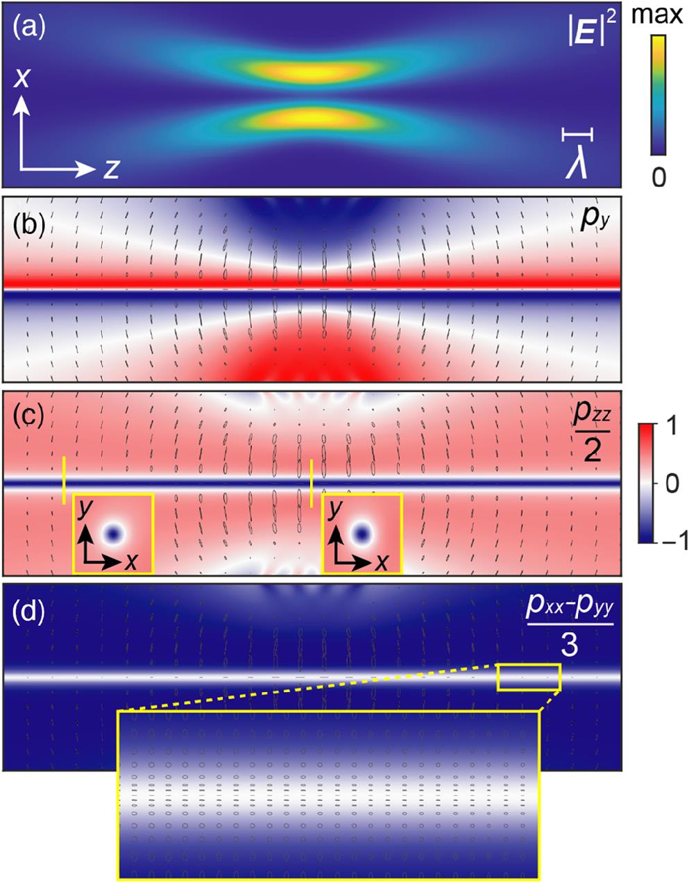
The ratio introduced in the previous section may be probed experimentally by measuring the polarization parameter . The independence of from the beam waist found in the previous section has immediate implications for which, as a result, maintains constant transverse spatial dimensions independently of beam divergence due to diffraction. Using Eq. (5) and the definitions from Eq. (8), -independent expressions can be obtained for for different beam polarizations For a circularly polarized beam with , it follows from Eq. (10) that in the vortex center and approaches unity with increasing radial distance to the singularity. Zero crossing () takes place at and is independent of both the beam waist and the propagation distance [see insets of Fig. 1(c)], while increasing linearly with . Similar propagation-independent expressions may be obtained for the other polarization parameters in Eq. (8) with playing the role of a scaling variable (see Appendix A for details).
Figure 1.Polarization parameters for a focused Laguerre–Gaussian vortex beam with l=1, linearly polarized along the direction and propagating along the axis. The beam waist is . (a) The intensity distribution of the beam in the () plane. (b–d) Colormaps of the (a) , (b) , and (d) polarization parameters with polarization ellipses overlaid on top, indicating the polarization state at each point in space. The polarization structure around the phase singularity is nondiffractive and invariant with respect to the beam waist. The inserts in (c) show the cross-sections at different positions. The insert in (d) shows the zoom near the beam centre.
The above results were obtained in a simplified analytical model for a paraxial optical vortex field. Next, we demonstrate the nondiffractive behavior of these polarization features using numerical simulations for a nonparaxial field.
4 Numerical Simulations and Discussion
We now outline a full-wave nonparaxial numerical approach. Any monochromatic electromagnetic field can be decomposed into a spectrum of plane-wave components with wave vectors lying on the -sphere of radius and hence , as follows: where are the components of the angular spectrum pertaining to each of the orthonormal polarization basis vectors, which we take as and , corresponding to the azimuthal and polar angle spherical basis vectors tangential to the -sphere.18–20 Equation (11) is an integration of plane waves and constitutes an exact solution to the Maxwell’s equations, including all the field components. To compute it, one only needs to find the spectral amplitudes corresponding to the desired illumination.
For these exact field calculations, we employ the Laguerre–Gaussian vortex beam widely used in singular optics.11 The angular spectrum of a Laguerre–Gaussian vortex beam can be calculated by selecting the plane and performing a Fourier transform .20,21 The derivation of the plane wave polarization amplitudes from the paraxial Laguerre–Gaussian beam field is described in detail in Appendix C.
We can use Eq. (11) to calculate the full 3D electric field and plot required polarization parameters without any approximations. The first example is a linearly polarized nonparaxial vortex beam with and propagating along the positive axis (Fig. 1). The tight focusing creates a highly divergent beam. In this case, the , , and parameters are required to fully describe the polarization structure [please note that the only remaining nonzero polarization parameter is but its behavior in the plane is the same as that of in the plane; see Fig. 1(b)]. In contrast to the electric field, which diffracts naturally after a propagation distance of just a few wavelengths [Fig. 1(a)], all three polarization parameters in Figs. 1(b)–1(d) clearly show no divergence around the phase singularity that lies on the axis. The polarization structures remain invariant and extend far beyond the focal plane, in agreement with the analytical paraxial predictions for in Eq. (5), but numerically observed here beyond the paraxial approximation.
We now demonstrate the equivalent polarization properties of a circularly polarized vortex beam. Figure 2(a) shows the intensity of a circularly polarized vortex beam, similar to the previous case except with , so that the spin and orbital angular momenta are antialigned. The polarization parameters again reveal a nondivergent polarization structure around the beam axis [Figs. 2(b)–2(d)]. For a vortex beam with a beam waist of double the size and, therefore, weaker focusing, the nondiffractive polarization structure near the phase singularity remains unperturbed, with the (white) contour lying at in both Figs. 2(d) and 2(h), in good agreement with the analytical result from Eq. (10): . This structural invariance has been observed for all beam waists, independent of focusing.
Figure 2.Polarization parameters for a focused Laguerre–Gaussian vortex beam with l=1and (left-hand circularly polarized), propagating along the positive axis. The beam waist is (a–d) and (e–h) . (a) and (e) The intensity distribution of the beam in the () plane. (b–d) and (f–h) Colormaps of the (b,f) , (c,g) , and (d,h) polarization parameters with polarization ellipses overlaid on top, indicating the polarization state at each point in space. The polarization structure around the phase singularity is nondiffractive and invariant with respect to the beam waist.
The main challenge in detecting this nondiffractive polarization property is the requirement to perform measurements in a region of space where the field intensity is weaker compared to its maximum. The ability to detect it is determined by the sensitivity of the detection apparatus, and can be mediated to some degree by the choice of wavelength, beam waist, how far the detection plane is from the focal plane, and what polarization structure is being investigated. Figure 3(a) shows the cross-sectional plots of the parameter for the linearly polarized vortex beam in Fig. 1 at different points along the axis. As before, we see nondiffractive behavior when near the beam centre, indicated by a horizontal dotted black line. Note how other features where at locations further away from the beam center are subjected to diffraction. The intensity of the normalized electric field in the same cross-sectional planes at the location of the nondiffracting polarization features, indicated by the vertical dotted black lines, is 37% of the peak intensity at the focal plane, and 2.8% at [Fig. 3(b)]. The polarization structure should, therefore, be easily detectable in the focal plane of the beam and measurable away from the focus. The intensity drop-off of a beam is dictated by the Rayleigh range, which is proportional to the square of the beam waist. However, increasing the beam waist reduces the intensity of the longitudinal field. The resulting optimization will depend on the measurement sensitivity and the desired application.
Figure 3.Cross sections of the linearly polarized vortex beams with depicted in Fig. 1 showing (a) and (b) at the focal plane and after propagating a distance of . The vertical dashed lines show the points at which and the corresponding field intensity for each cross-section plane.
To experimentally verify the propagation-invariant polarization structures, a vortex beam will likely need to be focused using a lens with a defined numerical aperture (NA). The effect of a restricted NA was simulated by limiting the integration of the () plane in Eq. (11) from to . Figure 4(a) shows the nonzero component of the angular spectrum for a linearly polarized vortex beam with and , obtained using Eq. (16), which is equivalent to the back focal plane image of the beam. The phase singularity is clearly visible at . In Figs. 1–3, all the fields within the light line (indicated by a green line) are integrated using Eq. (11) to create the real-space field distribution. We now crop the angular spectrum down to a factor of with , as indicated by the red dotted line. Figure 4(b) shows the intensity profile of the beam after this NA restriction. When compared with the ideal beam in Fig. 1(b), the polarization parameter of the restricted beam in Fig. 4(c) reveals the same nondiffractive property near the phase singularity and only disturbances in the peripheral fields are observed. As the NA is reduced further (not shown), the beam waist widens but the behavior around the phase singularity is maintained.
Figure 4.(a) The angular spectrum of a linearly polarized ( direction) vortex beam with l=1. The green line indicates the light line and the red dotted line indicates the inner limit of the cropped region dictated by the objective with . (b) The intensity distribution of the corresponding vortex beam with generated by integrating the field distribution in (a). The beam waist is . (c) Colormap of the polarization parameter with polarization ellipses overlaid on top, indicating the polarization state at each point in space. The nondiffractive behavior near the phase singularity is maintained and only peripheral fields are affected by the NA reduction. (d–f) The same quantities as in (a–c) but with part of the angular spectrum removed and astigmatism applied along direction.
One can proceed to add more imperfections or aberrations to the beam. A defect or a piece of dust on the focusing lens can perturb the beam. This can be approximated by deleting part of the angular spectrum. A lens can also introduce astigmatism to the beam. The effect can be roughly modeled by scaling and in the angular spectrum. Figure 4(d) shows the angular spectrum of the same vortex beam as Fig. 4(a) with a restricted NA of 0.5 but with these two additional perturbations applied. The angular spectrum is set to zero for and , and is transformed by , therefore, reciprocally stretching the beam in the direction. The nondiffractive nature of the polarization parameter near the phase singularity is preserved for such scattered focused beams with astigmatism [Fig. 4(f)]. We therefore conclude that the nondiffractive polarization structures within a vortex beam should be robust to a variety of experimental imperfections and experimentally observable in this respect.
When considering higher-order vortex beams, further complications can arise from beam imperfections, resulting in splitting the high-order vortex into multiple low-order vortices.22–24 This can impact the topology of the observed nondiffractive polarization structure as discussed in Appendix D.
5 Conclusions
We have studied the polarization of vector beams carrying optical angular momentum. We show the existence of polarization features within optical vortex beams that maintain constant transverse spatial dimensions independently of the beam divergence due to diffraction. The exact size of these vortex polarization structures is dictated by the presence of the longitudinal electric field in the beam, and such structures are expected for vortex beams of all topological charges. An analytical paraxial model predicts their presence in weakly focused beams and a numerical angular spectrum approach further extended this prediction to tightly focused beams, thereby proving applicability to all vortex beams. These polarization features are not affected by finite NAs and so should be experimentally measurable. It should be noted that the predicted nondiffractive polarization features have relatively small transverse dimensions of the order , centered on a low-intensity region of the optical vortex wavefront. Therefore, future measurements will require subwavelength resolution at low and increased sensitivity of the probe for larger values of .
The demonstrated effect allows one to pinpoint the position of a phase singularity with subwavelength accuracy independently of the size of a beam spot. This property may have useful applications in metrology, optical communications, optical networking, laser sensing, and radar operations.
6 Appendix A. Calculation of Polarization Parameters
In Table 1, we present analytic expressions for polarization parameters [Eq. (8)] calculated for different polarizations of optical vortex beams; is assumed. The transverse field is defined by Eq. (1), and the longitudinal field is obtained from combined with the paraxiality condition, Eq. (2), at radial positions near the beam axis (much smaller than the beam waist). As in the main text, we define the dimensionless radial parameter , which depends on the topological charge . The transverse polarization vector 𝛈 for different polarizations is given in terms of unit vectors in Cartesian or cylindrical coordinates.
Let us demonstrate the derivation in the case of linearly polarized (along the axis) light, so that 𝛈. The continuity equation , together with the paraxiality condition, gives us the longitudinal field from the transverse-field derivative: . After some algebra, the field derivative can be obtained as In the region much smaller than the beam waist , the second term in the parenthesis can be dropped, and the ratio of longitudinal-to-transverse field is The magnitude of this expression yields the result of Eq. (5). Using the definitions in Eq. (8), the linear polarization column in Table 1 can be obtained. The derivation is similar for other choices of a polarization vector 𝛈.
The expressions for circular polarization () are simplified in cylindrical coordinates, for which radial components of the polarization vector and tensor are zero: , , , and .
7 Appendix B. Definition of Stokes Parameters
A polarization coherence matrix for two-dimensional electric fields is defined in terms of Stokes parameters as16If the transverse electric field is linearly polarized along the axis, then the polarization of the full field is determined by three Stokes parameters defined for its corresponding components, which in turn relate to the polarization parameters in Eq. (8) as
8 Appendix C. Decomposing the Angular Spectrum into a Polarization Basis
Here, we show how nonparaxial fields of a focused vortex beam are calculated using the angular spectrum approach. We start with the paraxial expression for a Laguerre–Gauss beam11𝛈where is the beam waist in the focal plane, is the beam radius at any point in space, is the generalized Laguerre polynomial of order and a radial index , is the beam curvature radius, and is the Gouy phase factor. We then consider a Fourier transform in the plane that defines the angular spectrum of a beam: This Fourier transform can be solved analytically. For an and Laguerre–Gauss beam 𝛈This is the angular spectrum of the transverse components only (it ignores the component), but from one can find the plane wave amplitudes that, when substituted into Eq. (11), give an electric field at (the focal plane), whose transverse component matches exactly Eq. (14), but which also possesses the corresponding component that appears naturally from the electromagnetic plane-wave polarization superposition.
In the remainder of this section, we do not explicitly write the dependencies of the angular spectrum for ease of notation, but note that all the fields mentioned here are the spectra defined in the plane unless otherwise stated. All fields are assumed to be time-harmonic.
The angular spectrum of the total field can be represented in a Cartesian basis , which can be split into a transverse part and a longitudinal part . Similarly, in the polarization basis . Equating these, one can write the transverse part of the field as We can further write in terms of as , where we used the fact that because . Thus, the transverse field is uniquely related to the and polarization amplitudes as If we now perform a dot product with the p/s basis unit vectors, and noting that and , we find Knowing that , we find that and so we can obtain the orthogonal scalar plane-wave polarization coefficients in terms of the transverse field spectrum as Applied to the specific case of the vortex beam defined by Eq. (16), we obtain the explicit expressions for the polarization basis coefficients where 𝛈. The nonparaxial fields are then generated by substituting the above into Eq. (11) from the main text. We numerically evaluate the integral in Eq. (11) as a finite sum of different plane waves whose fields can be analytically computed and summed.
9 Appendix D. Splitting of Higher-Order Vortices
The analytical model in Sec. 2 is concerned with ideal vortex beams of any order. However, when a vortex beam with is perturbed, the high-order vortex can split into multiple lower-order vortices.
The splitting of an vortex beam can be investigated with our nonparaxial angular spectrum method by employing the appropriate equations for and . The continuous integration of the angular spectrum is approximated by a summation of a finite number of plane waves and inevitably generates a numerically approximate beam, which tends toward the ideal case when the number of plane waves tends to infinity. Figures 5(a)–5(d) show the phase of the transverse electric field for a nonparaxial vortex beam linearly polarized along , constructed using the angular spectrum approach and integrating a finite number of plane waves. This integration introduces a small perturbation in the fields away from the ideal vortex beam and, therefore, promotes a splitting of the singularity into three distinct vortices. The separation distance among the three singularities is reduced by increasing the number of plane waves.
Figure 5.(a–d) The phase of in the focal plane of a nonparaxial l=3 vortex beam linearly polarized along direction with and (e–g) the polarization parameter in a plane (to avoid focal plane features) simulated for different finite numbers of constituent plane waves (indicated in the panels). The l=3 vortex splits in three l=1 vortices with an increased splitting for a decreased .
This split vortex beam can now be analyzed by simulating polarization parameters in Eq. (8). For an obtained, simulated with high , nondiffractive features in the polarization structure can be observed similar to what was previously seen for an vortex [cf. Figs. 5(e) and 1(c)]. When is high, the individual vortices are extremely close together, and a collective polarization structure (such as the white cylindrical contour) is present. When is reduced and the vortices separate slightly, the contour is warped [Fig. 5(f)]. With further reduction of , the singularities move far apart and do not exhibit a collective polarization structure; instead, three individual cylindrical contours are observed [Fig. 5(g)]. In all three cases, the polarization structures were found to be nondiffractive as they extend far beyond the divergent beam field intensity drop-off. In other words, an ideal vortex beam exhibits the polarization structure predicted in Sec. 2 with the analytical paraxial model, but this structure breaks down into three separate structures when the beam is imperfect, with each of the separate vortices carrying its own non-diffractive polarization structure.
Andrei Afanasev received his PhD in physics from Karazin Kharkiv National University in Ukraine. Currently, he is working as a Gus Weiss professor of physics and endowed chair in theoretical physics at the Department of Physics in George Washington University in Washington DC, United States. His research interests include quantum electrodynamics, nuclear physics, and quantum optics.
Jack J. Kingsley-Smith received his MSc and PhD degrees in physics from the Department of Physics at King’s College London. Currently, he is a postdoctoral research associate at the same institution and is working on optical forces and structured light.
Francisco J. Rodríguez-Fortuño received his BSc, MSc, and PhD degrees at Universitat Politecnica de Valencia, Spain, with research stays at University of Pennsylvania and King’s College London, where he obtained a permanent academic position in 2015, starting his research team. He was a PI of ERC Starting Grant PSINFONI and Co-I in EIC Pathfinder CHIRALFORCE. Currently, he is working as a reader at King’s College London Physics Department, researching on nanophotonics and new electromagnetic phenomena, with a focus on near-field effects.
Anatoly V. Zayats is chair in experimental physics and head of the photonics and nanotechnology at the Department of Physics, King’s College London. He is working as a codirector at London Centre for Nanotechnology and London Institute for Advanced Light Technologies. His research interests include nanophotonics and plasmonics, metamaterials and metasurfaces, electromagnetic field topology and optical spin-orbit coupling, and nonlinear and ultrafast optics.
Andrei Afanasev, Jack J. Kingsley-Smith, Francisco J. Rodríguez-Fortuño, Anatoly V. Zayats, "Nondiffractive three-dimensional polarization features of optical vortex beams," Adv. Photon. Nexus 2, 026001 (2023)