• Photonics Research
  • Vol. 11, Issue 2, 299 (2023)
Guoqing Ma1、2, Junjie Yu1、2、3, Rongwei Zhu1、2, and Changhe Zhou1、2、*
Author Affiliations
  • 1Laboratory of Information Optics and Optoelectronic Technology, Shanghai Institute of Optics and Fine Mechanics, Chinese Academy of Sciences, Shanghai 201800, China
  • 2Center of Materials Science and Optoelectronics Engineering, University of Chinese Academy of Sciences, Beijing 100049, China
  • 3e-mail: Junjiey@siom.ac.cn
  • show less
    DOI: 10.1364/PRJ.472741 Cite this Article Set citation alerts
    Guoqing Ma, Junjie Yu, Rongwei Zhu, Changhe Zhou. Optical multi-imaging–casting accelerator for fully parallel universal convolution computing[J]. Photonics Research, 2023, 11(2): 299 Copy Citation Text show less
    Schematic of the optical multi-imaging–casting architecture: optical parallel convolution process with different convolutional strides s1 (a) and s2 (b); (c) optical architecture principle of OMica, where the beam splitter (BS) is a diffractive beam splitter; Oy is diffraction order in the y direction (indicated by different line types), and θ is the angle difference between any two adjacent diffraction orders in object space (θ1 and θ2 are diffraction angles of Oy =1 and Oy=2 diffraction orders, respectively); θ′ is the angle difference in image space (θ1′ and θ2′ are diffraction angles of Oy =1 and Oy=2 diffraction orders, respectively); d is the distance between matrix A and BS, and l is the distance between matrix B and the image of BS. a, b, and c are spot arrays corresponding to different diffraction orders diffracted from a BS. The imaging–casting system is composed of L1 and L2, with focal lengths f1 and f2. L3 is a focusing lens with focal length f3. s is the lateral shifts of the image of diffraction orders of DG on the SLM2 plane corresponding to the convolutional stride, and this convolutional stride could be tunable by changing the distance d [s1 and s2 correspond to different convolutional strides shown in (a) and (b)].
    Fig. 1. Schematic of the optical multi-imaging–casting architecture: optical parallel convolution process with different convolutional strides s1 (a) and s2 (b); (c) optical architecture principle of OMica, where the beam splitter (BS) is a diffractive beam splitter; Oy is diffraction order in the y direction (indicated by different line types), and θ is the angle difference between any two adjacent diffraction orders in object space (θ1 and θ2 are diffraction angles of Oy=1 and Oy=2 diffraction orders, respectively); θ is the angle difference in image space (θ1 and θ2 are diffraction angles of Oy=1 and Oy=2 diffraction orders, respectively); d is the distance between matrix A and BS, and l is the distance between matrix B and the image of BS. a, b, and c are spot arrays corresponding to different diffraction orders diffracted from a BS. The imaging–casting system is composed of L1 and L2, with focal lengths f1 and f2. L3 is a focusing lens with focal length f3. s is the lateral shifts of the image of diffraction orders of DG on the SLM2 plane corresponding to the convolutional stride, and this convolutional stride could be tunable by changing the distance d [s1 and s2 correspond to different convolutional strides shown in (a) and (b)].
    Procedure of converting the original grayscale matrix with negative elements into encoded matrices of NBD. (a) The encoding matrices are loaded into the OMica system to compute the convolution, with the experimental encoded convolutional result decoded into the original matrix. (b) Original grayscale matrices A and B, and original convolutional results matrix C. (c) Larger encoded matrices A and B in spatial sequence and the same size encoded convolutional results matrix C.
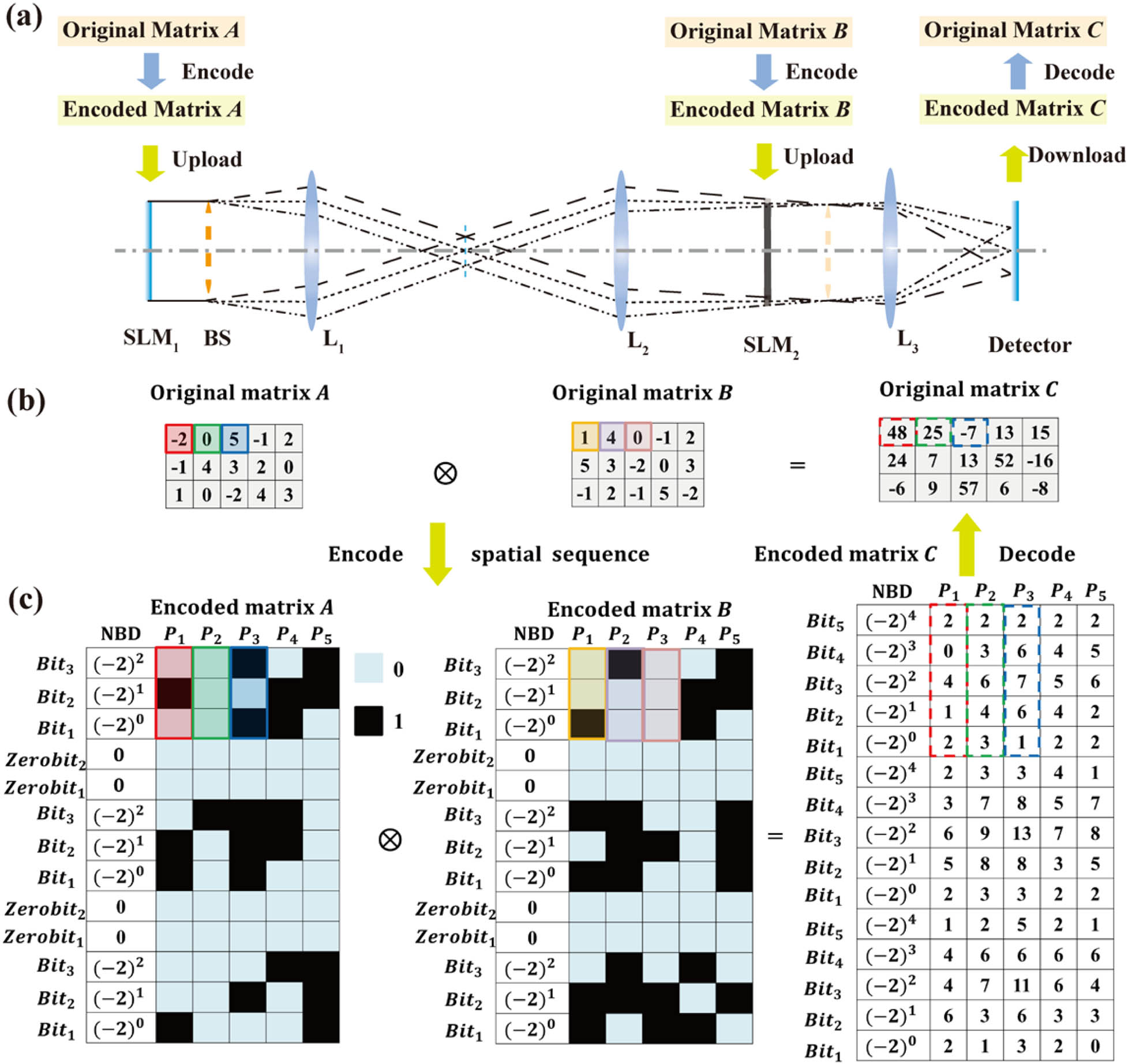
    Fig. 2. Procedure of converting the original grayscale matrix with negative elements into encoded matrices of NBD. (a) The encoding matrices are loaded into the OMica system to compute the convolution, with the experimental encoded convolutional result decoded into the original matrix. (b) Original grayscale matrices A and B, and original convolutional results matrix C. (c) Larger encoded matrices A and B in spatial sequence and the same size encoded convolutional results matrix C.
    Experimental results of hybrid analog–digital matrix convolution for two groups of matrices based on spatial sequence encoding. The subfigures from left to right are the light intensity distribution of the spot array denoting the convolution, theoretical convolutional values, experimental convolutional results, error map between theoretical and experimental results, and decoded convolutional results, respectively, in (a) matrices A1 and B1 and (b) matrices A2 and B2. The red cross marks the centroid positions of each spot.
    Fig. 3. Experimental results of hybrid analog–digital matrix convolution for two groups of matrices based on spatial sequence encoding. The subfigures from left to right are the light intensity distribution of the spot array denoting the convolution, theoretical convolutional values, experimental convolutional results, error map between theoretical and experimental results, and decoded convolutional results, respectively, in (a) matrices A1 and B1 and (b) matrices A2 and B2. The red cross marks the centroid positions of each spot.
    Experimental results of high-accuracy convolution for two groups of grayscale matrices. (a), (b) Randomly generated 8-bit grayscale 10×10 matrices A3 and B3, 8-bit grayscale 20×20 matrices A4 and B4, respectively. The subfigures from left to right show the light intensity distribution of the spot array denoting the convolution, theoretical convolutional values, experimental convolutional results, error map between theoretical and experimental results (the red circle indicates the computing accuracy at that point is less than 8 bit), and histogram of the error distribution, respectively. The comparison of experimental convolutional results expands into one-dimensional (1D) vectors and theoretical convolutional results.
    Fig. 4. Experimental results of high-accuracy convolution for two groups of grayscale matrices. (a), (b) Randomly generated 8-bit grayscale 10×10 matrices A3 and B3, 8-bit grayscale 20×20 matrices A4 and B4, respectively. The subfigures from left to right show the light intensity distribution of the spot array denoting the convolution, theoretical convolutional values, experimental convolutional results, error map between theoretical and experimental results (the red circle indicates the computing accuracy at that point is less than 8 bit), and histogram of the error distribution, respectively. The comparison of experimental convolutional results expands into one-dimensional (1D) vectors and theoretical convolutional results.
    Inference process for the convolutional neural network performed by OMica based on the MNIST dataset. (a) Execution of convolution operation by encoding each original convolutional kernel into high-bit and low-bit kernels; (b) schematic of the optical convolutional architecture performing CNN inference; (c) absolute error AE map comparing theoretical and experimental results of the convolution of a handwritten digit 7 as an input; confusion matrix of blind-testing 1000 images from the MNIST dataset when matrix convolutions are executed by the optical hardware (d) and by pure electric hardware (e). The purple box marks the first convolutional kernel to realize the whole process of encoding, convolution, and decoding.
    Fig. 5. Inference process for the convolutional neural network performed by OMica based on the MNIST dataset. (a) Execution of convolution operation by encoding each original convolutional kernel into high-bit and low-bit kernels; (b) schematic of the optical convolutional architecture performing CNN inference; (c) absolute error AE map comparing theoretical and experimental results of the convolution of a handwritten digit 7 as an input; confusion matrix of blind-testing 1000 images from the MNIST dataset when matrix convolutions are executed by the optical hardware (d) and by pure electric hardware (e). The purple box marks the first convolutional kernel to realize the whole process of encoding, convolution, and decoding.
    Schematic of the optical convolution experimental system using the DG. LED, light-emitting diode with wavelength λ=450 nm; M1–6, reflective aluminum mirrors; AP1,2,3, aperture pinholes; L1–5, convergent lenses; L6, L7, L10, Fourier transform lenses; PBS1,2,3, cube polarization beam splitters; SLM1, SLM2, reflected liquid crystal SLMs; APA, aperture array; DG, Dammann grating; BS, non-polarizing beam splitter; sCMOS1, scientific complementary metal–oxide–semiconductor camera for detection; CMOS2, CMOS camera for monitoring. I, II, III, and the plane of the square aperture are one group of object–image conjugate planes. IV and V are other groups of object–image conjugate planes. Plane V is the image plane of the DG. d0 is the characteristic distance corresponding to s=1, which can be adjusted to match the physical size of the matrix unit of matrix B to the different stride size.
    Fig. 6. Schematic of the optical convolution experimental system using the DG. LED, light-emitting diode with wavelength λ=450  nm; M16, reflective aluminum mirrors; AP1,2,3, aperture pinholes; L15, convergent lenses; L6, L7, L10, Fourier transform lenses; PBS1,2,3, cube polarization beam splitters; SLM1, SLM2, reflected liquid crystal SLMs; APA, aperture array; DG, Dammann grating; BS, non-polarizing beam splitter; sCMOS1, scientific complementary metal–oxide–semiconductor camera for detection; CMOS2, CMOS camera for monitoring. I, II, III, and the plane of the square aperture are one group of object–image conjugate planes. IV and V are other groups of object–image conjugate planes. Plane V is the image plane of the DG. d0 is the characteristic distance corresponding to s=1, which can be adjusted to match the physical size of the matrix unit of matrix B to the different stride size.
    Photographs of the experiment system of OMica. (a) Entire optical system; (b) SLM mounted on a 4D manual stage for loading kernel A, (c) SLM mounted on a 4D manual stage for loading matrix B, and (d) enlarged part of the sCMOS1 detector and monitoring CMOS2 camera.
    Fig. 7. Photographs of the experiment system of OMica. (a) Entire optical system; (b) SLM mounted on a 4D manual stage for loading kernel A, (c) SLM mounted on a 4D manual stage for loading matrix B, and (d) enlarged part of the sCMOS1 detector and monitoring CMOS2 camera.
    Typical patterns loaded onto two SLMs for alignment. (a) Alignment pattern and (b) square array pattern.
    Fig. 8. Typical patterns loaded onto two SLMs for alignment. (a) Alignment pattern and (b) square array pattern.
    Experimental results for demonstration of kernel sliding. (a), (b) Images loaded onto two SLMs. (c)–(j) Images captured by the monitoring CMOS2 camera as the iris moves from left to right, allowing only one diffraction order to pass through its aperture in sequence.
    Fig. 9. Experimental results for demonstration of kernel sliding. (a), (b) Images loaded onto two SLMs. (c)–(j) Images captured by the monitoring CMOS2 camera as the iris moves from left to right, allowing only one diffraction order to pass through its aperture in sequence.
    1×20 (a) and 1×28 (b) DG beam splitting order normalized energy distribution.
    Fig. 10. 1×20 (a) and 1×28 (b) DG beam splitting order normalized energy distribution.
    Intensity and angle distribution of 20×28 2D DG. (a) Simulation result of intensity distribution versus different orders; (b) simulation result of diffraction angle versus diffraction order; (c) intensity map of the spot array captured in the experiment (the cross represents the centroid); (d) experimental results of normalized intensity distribution versus diffraction order.
    Fig. 11. Intensity and angle distribution of 20×28 2D DG. (a) Simulation result of intensity distribution versus different orders; (b) simulation result of diffraction angle versus diffraction order; (c) intensity map of the spot array captured in the experiment (the cross represents the centroid); (d) experimental results of normalized intensity distribution versus diffraction order.
    Experimental convolutional results for 180×224 matrices. (a)–(c) Theoretical convolutional results, experimental convolutional results, and experimental detection light distribution, respectively; (d) partially enlarged view of the experimental light spot on (c); (e) error distribution; (f) proportion of experimental light intensity distribution.
    Fig. 12. Experimental convolutional results for 180×224 matrices. (a)–(c) Theoretical convolutional results, experimental convolutional results, and experimental detection light distribution, respectively; (d) partially enlarged view of the experimental light spot on (c); (e) error distribution; (f) proportion of experimental light intensity distribution.
    Schematic of the CNN architecture.
    Fig. 13. Schematic of the CNN architecture.
    Learning curve of the CNN.
    Fig. 14. Learning curve of the CNN.
    Typical error maps between convolutional results obtained from the optical hardware and that of an electrical computer with the full precision of different input handwritten digits (from 0 to 9) for these 10 convolutional kernels after encoding.
    Fig. 15. Typical error maps between convolutional results obtained from the optical hardware and that of an electrical computer with the full precision of different input handwritten digits (from 0 to 9) for these 10 convolutional kernels after encoding.
    Guoqing Ma, Junjie Yu, Rongwei Zhu, Changhe Zhou. Optical multi-imaging–casting accelerator for fully parallel universal convolution computing[J]. Photonics Research, 2023, 11(2): 299
    Download Citation