• Photonics Research
  • Vol. 9, Issue 10, 1898 (2021)
Kewei Liu1, Xiaosheng Xiao2、4、*, Yihang Ding1, Hongyan Peng3, Dongdong Lv3, and Changxi Yang1、5、*
Author Affiliations
  • 1State Key Laboratory of Precision Measurement Technology and Instruments, Department of Precision Instruments, Tsinghua University, Beijing 100084, China
  • 2State Key Laboratory of Information Photonics and Optical Communications, School of Electronic Engineering, Beijing University of Posts and Telecommunications, Beijing 100876, China
  • 3School of Physics and Electronic Engineering, Hainan Normal University, Haikou 571158, China
  • 4e-mail: xsxiao@bupt.edu.cn
  • 5e-mail: cxyang@tsinghua.edu.cn
  • show less
    DOI: 10.1364/PRJ.428687 Cite this Article Set citation alerts
    Kewei Liu, Xiaosheng Xiao, Yihang Ding, Hongyan Peng, Dongdong Lv, Changxi Yang. Buildup dynamics of multiple solitons in spatiotemporal mode-locked fiber lasers[J]. Photonics Research, 2021, 9(10): 1898 Copy Citation Text show less
    Experimental setup of the STML fiber laser and system of DFT for real-time measurement. LD, laser diode; SPDM, short-pass dichroic mirror; L1, L2, lens; M, mirror; ISO, isolator; SF, spectral filter; HWP, half-wave plate; QWP, quarter-wave plate; PBS, polarization beam splitter; BS, beam splitter; YDFA, ytterbium-doped fiber amplifier; ODL, optical delay line; PD, photodetector.
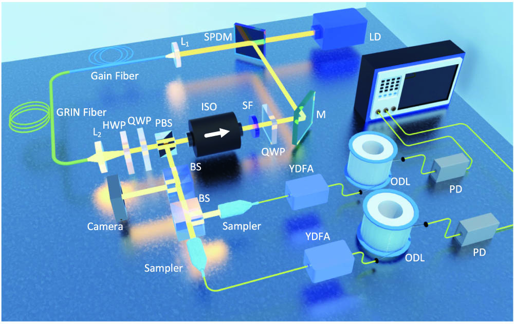
    Fig. 1. Experimental setup of the STML fiber laser and system of DFT for real-time measurement. LD, laser diode; SPDM, short-pass dichroic mirror; L1, L2, lens; M, mirror; ISO, isolator; SF, spectral filter; HWP, half-wave plate; QWP, quarter-wave plate; PBS, polarization beam splitter; BS, beam splitter; YDFA, ytterbium-doped fiber amplifier; ODL, optical delay line; PD, photodetector.
    Buildup dynamics of a three-pulse STML. (a) Experimental recordings of the multipulse buildup of two channels, I (orange) and II (blue), which are simultaneously acquired via two spatial sampling points. The two figures in the right panel exhibit the stretched pulse profiles at approximately 2500 μs within one cavity round-trip time (∼31.1 ns), indicating diverse spectral profiles between two different channels. The inset shows the corresponding beam profile after steady mode locking, where the sampling positions of channels I and II are indicated by the red circles and white arrows. (b) Contour plot of the extracted experimental data ranging over 58,000 round trips. The figure in the right panel displays the close-up evolution (indicated by the white dashed rectangle in the figure on the left) near the establishment of mode-locked pulses. (c) Corresponding total energy evolution integrated within each round trip. The insets exhibit the zoom-in energy variation during the turbulent period [indicated by the white dashed rectangle and arrow on the right panel of (b)] of the buildup process. (d) Integrated energy of each stretched pulse (pulse 1, pulse 2, and pulse 3) of channels I and II after entering the stable STML state. The line graph shows the energy ratio of each stretched pulse between two different channels.
    Fig. 2. Buildup dynamics of a three-pulse STML. (a) Experimental recordings of the multipulse buildup of two channels, I (orange) and II (blue), which are simultaneously acquired via two spatial sampling points. The two figures in the right panel exhibit the stretched pulse profiles at approximately 2500 μs within one cavity round-trip time (31.1  ns), indicating diverse spectral profiles between two different channels. The inset shows the corresponding beam profile after steady mode locking, where the sampling positions of channels I and II are indicated by the red circles and white arrows. (b) Contour plot of the extracted experimental data ranging over 58,000 round trips. The figure in the right panel displays the close-up evolution (indicated by the white dashed rectangle in the figure on the left) near the establishment of mode-locked pulses. (c) Corresponding total energy evolution integrated within each round trip. The insets exhibit the zoom-in energy variation during the turbulent period [indicated by the white dashed rectangle and arrow on the right panel of (b)] of the buildup process. (d) Integrated energy of each stretched pulse (pulse 1, pulse 2, and pulse 3) of channels I and II after entering the stable STML state. The line graph shows the energy ratio of each stretched pulse between two different channels.
    Buildup dynamics of STML soliton bunch composed of 23 pulses. To avoid overlap, the pulses are not stretched. (a) Contour plot of the buildup process covering 60,000 round trips; (b) close-up of the soliton bunch generation, indicated by the white dashed rectangle in (a). There appear multiple small peaks that seed mode-locked pulses afterwards in channel II. While in channel I, these tiny peaks are barely observed. Note the buildup of different pulses is asynchronous. The maximum buildup time difference is around 50 round trips.
    Fig. 3. Buildup dynamics of STML soliton bunch composed of 23 pulses. To avoid overlap, the pulses are not stretched. (a) Contour plot of the buildup process covering 60,000 round trips; (b) close-up of the soliton bunch generation, indicated by the white dashed rectangle in (a). There appear multiple small peaks that seed mode-locked pulses afterwards in channel II. While in channel I, these tiny peaks are barely observed. Note the buildup of different pulses is asynchronous. The maximum buildup time difference is around 50 round trips.
    Basic model and typical result of multiple-soliton generation. (a) Schematic of the iterative model to simulate multipulsing STML. The interactions among transverse modes in the gain media are neglected; thus the modes are amplified as a whole in the gain media. The SA is mode-dependent and transverse mode decomposition and composition are implemented before and after the SA, respectively. (b) Calculated energy of the pulses (pulse 1, pulse 2, pulse 3) for different transverse modes (mode 1, mode 2, and mode 3) versus the saturable energy Esat (Esat is closely related to the pump power). TH1, TH2, and TH3 are the thresholds of pulse 1, pulse 2, and pulse 3, respectively.
    Fig. 4. Basic model and typical result of multiple-soliton generation. (a) Schematic of the iterative model to simulate multipulsing STML. The interactions among transverse modes in the gain media are neglected; thus the modes are amplified as a whole in the gain media. The SA is mode-dependent and transverse mode decomposition and composition are implemented before and after the SA, respectively. (b) Calculated energy of the pulses (pulse 1, pulse 2, pulse 3) for different transverse modes (mode 1, mode 2, and mode 3) versus the saturable energy Esat (Esat is closely related to the pump power). TH1, TH2, and TH3 are the thresholds of pulse 1, pulse 2, and pulse 3, respectively.
    Various multipulsing STML regimes containing different numbers of solitons. (a) Second-harmonic mode locking; (b) eight-soliton STML with equal pulse intensity; (c), (d) multiple-soliton STML with unequal pulse intensities; (e), (f) soliton bunches. The insets are the close-up of the pulses within one cavity FSR (∼31.1 ns).
    Fig. 5. Various multipulsing STML regimes containing different numbers of solitons. (a) Second-harmonic mode locking; (b) eight-soliton STML with equal pulse intensity; (c), (d) multiple-soliton STML with unequal pulse intensities; (e), (f) soliton bunches. The insets are the close-up of the pulses within one cavity FSR (31.1  ns).
    (a)–(b) 26th-order harmonic STML state. The waveform is displayed in (a) with the inset showing the beam pattern. The first highest peak of (b) the RF spectrum is at approximately 834 MHz (26 times of the cavity FSR), possessing around 25.9 dB prominence to the highest side peak. (c), (d) two-soliton STML. The temporal waveform and spectrum are shown in (c) and (d), respectively. (e), (f) Soliton-molecule STML: (e) spectrum (inset is the beam profile); (f) autocorrelation trace.
    Fig. 6. (a)–(b) 26th-order harmonic STML state. The waveform is displayed in (a) with the inset showing the beam pattern. The first highest peak of (b) the RF spectrum is at approximately 834 MHz (26 times of the cavity FSR), possessing around 25.9 dB prominence to the highest side peak. (c), (d) two-soliton STML. The temporal waveform and spectrum are shown in (c) and (d), respectively. (e), (f) Soliton-molecule STML: (e) spectrum (inset is the beam profile); (f) autocorrelation trace.
    Validation of STML of the multiple solitons in the multimode fiber laser cavity. (a) RF spectrum (inset, wide-range RF signal); (b) spectra extracted from three spatial positions A, B, C, denoted in the beam profile (the inset); (c) spectra of the entire output and the spectral-filtered outputs after the short-pass filter (filter 1) and long-pass filter (filter 2) with the corresponding beam profiles in the right column.
    Fig. 7. Validation of STML of the multiple solitons in the multimode fiber laser cavity. (a) RF spectrum (inset, wide-range RF signal); (b) spectra extracted from three spatial positions A, B, C, denoted in the beam profile (the inset); (c) spectra of the entire output and the spectral-filtered outputs after the short-pass filter (filter 1) and long-pass filter (filter 2) with the corresponding beam profiles in the right column.
    Buildup dynamics of a four-soliton STML. (a) Real-time experimental data acquired from channel I (orange) and channel II (blue); (b) corresponding stretched pulse waveforms after stable STML within one cavity FSR (∼31.1 ns); (c) overall energy variation during the buildup process. The selected data ranges are denoted by the black dashed rectangle in (a). The insets are the zoom-in waveforms showing the turbulent phase. (d) 2D contour plot of the four-soliton buildup process. The white dashed rectangles in (i) and (ii) refer to (c), the zoom-in figures exhibiting the establishment of the multiple-soliton in the right column. (e) Integrated pulse energy of channel I (orange) and channel II (blue). The ratios of pulse energy between two channels for each pulse are drawn with the black dashed line.
    Fig. 8. Buildup dynamics of a four-soliton STML. (a) Real-time experimental data acquired from channel I (orange) and channel II (blue); (b) corresponding stretched pulse waveforms after stable STML within one cavity FSR (31.1  ns); (c) overall energy variation during the buildup process. The selected data ranges are denoted by the black dashed rectangle in (a). The insets are the zoom-in waveforms showing the turbulent phase. (d) 2D contour plot of the four-soliton buildup process. The white dashed rectangles in (i) and (ii) refer to (c), the zoom-in figures exhibiting the establishment of the multiple-soliton in the right column. (e) Integrated pulse energy of channel I (orange) and channel II (blue). The ratios of pulse energy between two channels for each pulse are drawn with the black dashed line.
    Dynamics of the buildup of a three-soliton STML, including a pulsation process. (a) 2D contour plot showing the buildup dynamics of the three-soliton STML. The white circles highlight the pulse evolution distinction between the two channels during RO. (b) Zoom-in figures displaying the details near the soliton establishments. The white arrows denote the moments when the solitons rise up or annihilate. (c) Zoom figures of the pulsation process. The insets are the magnified figures showing the spectral evolution, extracted from a certain round-trip range denoted by the white rectangles. (d) Corresponding overall energy variation versus round trip. The insets are the zoom-in figures exhibiting the pulsation (breathing) behavior. (e) Stretched pulse profiles of channels I and II after steady mode locking; (f) integrated pulse energy. The dashed line represents the ratios of pulse energy between the two channels for each pulse.
    Fig. 9. Dynamics of the buildup of a three-soliton STML, including a pulsation process. (a) 2D contour plot showing the buildup dynamics of the three-soliton STML. The white circles highlight the pulse evolution distinction between the two channels during RO. (b) Zoom-in figures displaying the details near the soliton establishments. The white arrows denote the moments when the solitons rise up or annihilate. (c) Zoom figures of the pulsation process. The insets are the magnified figures showing the spectral evolution, extracted from a certain round-trip range denoted by the white rectangles. (d) Corresponding overall energy variation versus round trip. The insets are the zoom-in figures exhibiting the pulsation (breathing) behavior. (e) Stretched pulse profiles of channels I and II after steady mode locking; (f) integrated pulse energy. The dashed line represents the ratios of pulse energy between the two channels for each pulse.
    Schematic of the numerical simulation model of multiple-soliton with multiple modes.
    Fig. 10. Schematic of the numerical simulation model of multiple-soliton with multiple modes.
    Kewei Liu, Xiaosheng Xiao, Yihang Ding, Hongyan Peng, Dongdong Lv, Changxi Yang. Buildup dynamics of multiple solitons in spatiotemporal mode-locked fiber lasers[J]. Photonics Research, 2021, 9(10): 1898
    Download Citation