Soybean (Glycine max L.) is the world's most common oil-bearing crop and an important protein source for human populations, playing an essential role in global economic development (Tomar et al., 2009; Hellal and Abdelhamid, 2013; Das and Parida, 2014). Roughly two-thirds of the world's population does not consume enough protein. To balance population growth with protein needs, many countries have recently tried to increase soybean yields and planting areas (Li et al., 2019). Planting areas for soybeans in China are the most widespread after those for corn, rice, wheat, and potatoes. Soybean crops are also the most economically efficient and import intensive crops. Therefore, the soybean is an important basic and strategic material and occupies an extremely important position in China's national economy. The No.1 document of 2019 issued by Central Committee of the CPC describes the “implementation of a soybean and dairy revitalization plan” as one of the ten key objectives and calls to expand soybean planting areas; promote the demonstration and popularization of new varieties, technologies, and forms of mechanization; stabilize grain production; and improve subsidies for soybean producers. Northeastern China is one of the country's main soybean producing areas. Planting areas and yields in northeastern China are among the highest in the country, accounting for 1/3 of national soybean planting areas and yields and thus playing an important role in food production in China (Liu et al., 2008; Yang et al., 2020).

In terms of global warming, however, warming trends of the crop growing season have not been obvious. The crop planting belt has shifted north while varieties ripening later have increasingly extended their reach in recent years (Liu et al., 2016a; Fang et al., 2019). As a result, chilling injury is the most frequent agricultural problem experienced in northern China, resulting in the most serious yield losses (Han et al., 2010; Hao et al., 2010). From 1951 to 1980, eight severe cold periods occurred, three of which (1969, 1972, and 1976) resulted in yield losses of roughly 5.78 billion kg (Zhang et al., 2012). Soybeans grown in the northeast at high latitudes suffered more severe and frequent cases of chilling injury than those in other areas (Zhou et al., 2017). Due to the insufficient supply of heat and considerable temperature variations in northeastern China, soybean can suffer a series of problems throughout the growing period, i.e., the delay of the growth period, dysplasia, empty shells, and chaff grains, reducing soybean yield and quality and economic losses. Therefore, it is essential to monitor chilling injury occurrence and evaluate yield losses of soybean crops in northeastern China (Liu et al., 2012).

Several recent studies have monitored chilling injury and assessed yield losses mainly using crop modelling and remote sensing monitoring. The calibrated crop model can also be used to simulate chilling injury scenarios at the field level. While these methods are easily applied at the field level, inferring to larger areas has limited validity due to a need of extensive and detailed information (e.g., variety characteristics, climate variables, soil conditions, and field management and cultivation methods). While these data are easily available at the field level, errors are inevitable when using field-level data for regional estimations due to high levels of spatial heterogeneity (Sinclair et al., 1993). Remote sensing monitoring, the constructed vegetation index and the temperature index mainly focus on distinguishing occurrences and levels of chilling injury. In addition, chilling injury indices and ground-based yield measurements collected in years with natural disasters are used to establish empirical relationships. However, while remote sensing monitoring can explain over 80% of yield variations among individual fields (Sinclair et al., 1993; Liu et al., 2016b), it is difficult to extrapolate these equations to new locations or years due to their limited spatial generalizability. In addition, while numerous studies have focused on impacts of chilling injury on corn and rice crops in northeastern China (Liu et al., 2016b; Chen, 2017), few have explored the impacts of chilling injury on soybeans in the same region. The above limitations highlight the need to develop more general means to quickly and accurately evaluate the effects of chilling injury on soybean crops.

Yield loss assessments, coupling crop models and remote sensing monitoring have been major issues of focus in recent years. The Google Earth Engine (GEE), with its powerful data storage and cloud computing capabilities, allows for the free sharing of image data (Gorelick et al., 2017) and the CROPGRO-Soybean model can dynamically and intuitively simulate soybean growth, development, and yields. These new tools allow for soybean growth monitoring and disaster loss assessment at high spatiotemporal resolutions (Boote et al., 2003). Using the GEE platform and crop model, we develop a fast, accurate, and cross-regional method for evaluating the impacts of chilling injury on soybean yields in northeastern China. We first optimize parameters of a localized soybean model, simulate cold injury scenarios to construct soybean chilling injury vulnerability models, and then spatialize yield loss mapping at a high resolution. Finally, yield losses at the county level are used to evaluate the performance of the proposed technique. Our aim is to provide a new method of soybean yield estimation and disaster loss assessment.

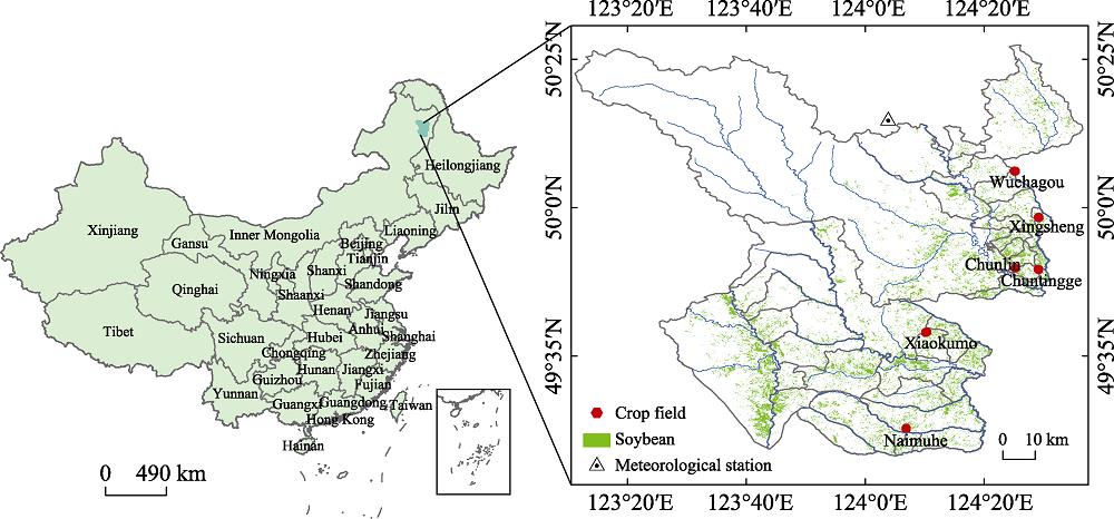
Oroqen Autonomous Banner, lying between 48°50′-51°25′N and 121°55′-126°10′E, is located between the Da Hinggan Mountains and Hulun Beir Grassland. It covers an area of approximately 6×10⁴ km² with roughly 2.1×10³ km² of cultivated land. The local terrain, which includes plateaus, mountains, and hills, forms a typical plateau landscape. The study area is characterized by a sub-humid warm temperate continental monsoon climate with four distinct seasons. Average annual temperatures range from -2.7℃ to 0.8℃ and increase from west to east. Temperatures can reach as low as -30℃ in January and as high as 37.5℃ in July with average temperatures ranging from 17.9℃ to 19.8℃. Approximately 95 d in the year are frost-free. Annual precipitation reaches 459.3-493.4 mm. Moreover, wind speeds are relatively low at 1.8 to 2.9 m/s. The Oroqen area serves as a major grain producer in the Inner Mongolian Autonomous Region with an average annual production level of 200 million kg. Soybean is the most common crop grown in this region (Figure 1).

2.2.1 Satellite data

Remote sensing has been widely used for crop growth monitoring and yield prediction, as it rapidly, macroscopically, and dynamically captures a wide range of data on the earth's surface through various bands (Chen et al., 2016). The Landsat 5 and Sentinel-2A surface reflectance products were first preprocessed on the GEE platform, i.e., radiation, geometric, and atmospheric correction. We then selected all available images visualizing critical soybean growth stages (i.e., May-September) using JavaScript API, including Landsat 5 images for 1984 to 2012 with a 30-m resolution and 16-d repeat and Sentinel-2A images for 2017 to 2019 with a 10-m resolution and 5-d repeat. Their quality control (QA) bands were used to remove effects of clouds using codes for Landsat 5 and Sentinel-2A images available at https://code.earthengine.google.com/dc10f7a140c2fe51aa30dfab08 and https://code.earthengine.google.com/6c7863acf90a59607fd4ec2cd6beadde, respectively. After the above processing, we obtained the spectral curve and calculated the vegetation index with good fit to the ground-based curve measures.

2.2.2 Meteorological and soil data

Daily climate data for 1981 to 2018, including those for average, maximum and minimum temperature (℃); rainfall (mm); and sunshine hours (h), were obtained from the National Meteorological Information Centre (https://data.cma.cn/en). Solar radiation levels were calculated according to previous research (Angstrom et al., 1924). Soil data used for the crop model are available from the Chinese soil science database (http://vdb3.soil.csdb.cn/) and include data on bulk density; organic carbon; total nitrogen; pH; and percentages of silt, sand, and clay. Soil albedo, runoff potential, and drainage rate values were also estimated (Jones et al., 2003). The soil fertility factor (SLPF) was set as 1.0, and the initial soil moisture content level was set as the field moisture capacity.

Daily climate data for 1981 to 2018, including those for average, maximum and minimum temperature (℃); rainfall (mm); and sunshine hours (h), were obtained from the National Meteorological Information Centre (https://data.cma.cn/en). Solar radiation levels were calculated according to previous research (Angstrom et al., 1924). Soil data used for the crop model are available from the Chinese soil science database (http://vdb3.soil.csdb.cn/) and include data on bulk density; organic carbon; total nitrogen; pH; and percentages of silt, sand, and clay. Soil albedo, runoff potential, and drainage rate values were also estimated (Jones et al., 2003). The soil fertility factor (SLPF) was set as 1.0, and the initial soil moisture content level was set as the field moisture capacity.

2.2.3 Land use and field measurement data

Six ground-based field measures for 2014 to 2017 for model calibration and localization and a soybean planting area map of Oroqen with a 10-m resolution were obtained from a local insurance company. As shown in Tables 1 and 2, ground-based field data used mainly include location data, basic information on soybean crops (e.g., variety maturity, yield, cultivar, and development period), and field management data (tillage, weeding, irrigation, fertilization, etc.). Recorded Oroqen soybean yields at the county level were obtained from the Department of Plantation Management (http://www.zzys.moa.gov.cn) and the Statistical Yearbook for Inner Mongolia for 1981 to 2017 (http://www.stats.gov.cn). River and administrative divisions were derived from the Resource and Environment Data Cloud Platform (http://www.resdc.cn). Finally, projections of all data were uniformly converted to WGS-1984 form.

Chilling injury assessment first involves determining historical cold years. According to previous research (Pang et al., 1983), two conditions should be met: (1) total Growing Degree Days (GDD), i.e., the mean daily temperature of above 10℃ for the growth period in a given year is less than 100℃ that of the historical mean soybean growth stage, and (2) lower soybean yields in the current year than in the preceding normal year (Pang et al., 1983). In this research, we only focus on identifying historical cold years and do not distinguish the degree of chilling injury. Years with GDD with temperatures below the historical mean of -100℃ include 1989, 1991, 1995, 2003, 2009, and 2018 (Figure 2), which is consistent with previous research (Zhang, 2017). However, no soybean yield losses occurred in Oroqen in 1991. Therefore, we only use 1989, 1995, 2003, 2009, and 2018 as historical cold years. Meanwhile, the preceding years within the study period (i.e., 1988, 1994, 2002, 2008, and 2017) are selected as normal years for our comparative analysis.

The CROPGRO-Soybean model available through DSSAT 4.7 has been widely used to simulate soybean growth and development around the world (Wang et al., 1995; Zhu et al., 2008). In the CROPGRO-Soybean model, 15 genetic parameters can determine a soybean cultivar (Table 3). In this study, ground-based field measurements for 2014 to 2017 were used to adjust optimal parameters and then for model localization. First, genetic parameters were initialized, and the number of iterations was set as 6000. Soybean variety parameters were calculated based on the GLUE (Generalized Uncertainty Estimation) module of the DSSAT model. Specifically, field measurements for 2014 to 2015 were used for model calibration, and those for 2016 to 2017 were used for model testing. The genetic parameters of six crop fields were then successively simulated. Finally, Root Mean Square Error (RMSE) and Relative Root Mean Square Error (RRMSE) tests were used to estimate deviation between the simulated and observed variables (i.e., flowering date, maturity date, and yield).

Yield loss assessment involves five steps: (1) simulating different combinations of cold and local field management scenarios based on the localized CROPGRO-Soybean model and then recording the simulated yield, daily Leaf Area Index (LAI), and the corresponding date (Day of year, DOY); (2) calculating GDD of each simulation scenario and then subtracting the mean number of GDD occurring from 1981 to 2018, namely, as Cold Degree Days (CDD); (3) constructing a vulnerability model of chilling injury from the simulated yield, CDD, and any combination of two LAIs for the critical growth period; (4) retrieving the actual LAI and acquisition date (DOY) of soybean planting grids on the GEE platform and calculating the actual number of CDD based on meteorological data; and (5) calculating the yield reduction rate on a pixel-by-pixel basis using the best available observation dates for each pixel.

3.3.1 Simulation of cold injury scenarios

A calibrated model can better simulate the impacts of climatic factors on crop growth and development and assess yield loss (Pang, 2015). In this study, a series of combined parameters of different sowing dates and planting densities was first generated. According to local field management records, sowing dates are set at equal intervals (5 d) from May 1st to June 6th and include May 1st, 6th, 11th, 16th, 22th, and 27th and June 1st and 6th. Planting densities were randomly generated at between 19.42 and 52.36 plants/m², including values of 19.42, 22.77, 31.82, 35.86, 38.87, 41.06, 47.43, and 52.36 plants/m². We also set up normal weather scenarios and seven cold injury scenarios: (1) three cold injury scenarios with daily temperature reductions of 1-3℃ across growth stages and (2) four other cold injury scenarios set randomly at a minimum temperature of 0℃ for 5 consecutive days from seedling emergence to the flowering stage, from the pod bearing stage to the pod bearing stage, and from the pod bearing stage to the mature stage. For each soybean field, we have 512 (8*8*8) simulation scenarios. Finally, the daily LAI and corresponding simulated yield of all soybean fields in the growth stage were recorded for analysis.

3.3.2 Calculating the chilling injury index

Effective accumulated temperatures exceeding 10℃ during the soybean growth periods of the simulation scenarios were calculated. Namely, the number of GDD and CDD was calculated by subtracting the mean number of GDD occurring in growth periods from 1981 to 2018. This CDD index was then used to determine the impact of chilling injury on final yields (Ma et al., 2003). Since the sowing dates and weather conditions are different for each simulation, the CDD values calculated from each simulation are also different. The CDD calculation formula is as follows:

where CDD is the effective accumulated temperature anomaly obtained from each simulation, D is the average daily temperature exceeding 10℃ on day i of the simulation growth period, n is the length of each simulation growth period, and $\overline{GDD}$ is the average effective accumulated temperature value of larger than 10℃ during the same period from 1980 to 2018.

3.3.3 Constructing vulnerability models of chilling injury

We expanded our analysis to 40 d before and after the soybean flowering date to create early and late windows. The simulated yields of 512 combination scenarios for six crop fields (6*512) were used as the dependent variable, and any two LAIs from the early and late windows and CDD were used as independent variables to construct multiple regression equations. A total of 1600 (40*40) equations were established.

where Yield represents the output of each simulation and LAI_1,d and LAI_2,d denote the LAI d days from the early window and late window, respectively. CDD represents the cool injury index for each simulation. β₀, β₁, β₂, and β₃ represent the regression coefficients of the constant, the LAI of the early window, the LAI of the late window, and CDD, respectively. Because the dates of usable imagery may differ by location and year and particularly for optical imagery for which cloud cover can vary by pixel, we compute regressions for an arbitrary number of combinations of image dates. Finally, we store the resulting coefficients for further analysis.

3.3.4 Estimations of yield loss in cold years

Previous studies have shown that the Wide Dynamic Range Vegetation Index (WDRVI) is sensitive to variations in the LAI and is closely related to the LAI (Anthony et al., 2012). Therefore, we first use the GEE platform to extract the maximum WDRVI and DOY of the early and late windows on a pixel-by-pixel basis and convert the WDRVI into the actual LAI of soybean planting grids (Lobell et al., 2015). We then apply regression equations to actual measurements obtained from satellite data (i.e., the actual LAI calculated from the WDRVI and DOY). This can generally be done on a pixel-by-pixel basis using the maximum WDRVI and DOY of the early and late windows for each pixel. The final step is to estimate yield and reduction rate at the pixel level and then generate yield estimations and yield reduction maps with a high resolution (i.e., 10 or 30 m). Due to a lack of other field measurements, we calculate the county-level yield and yield reduction rate from the mean of the pixel yield and reduction rate and use the recorded county-level yield to evaluate the performance of our proposed technique when applied to the Oroqen area. The yield reduction rate is expressed as “(the annual yield of a normal year - the annual yield of a cold year)/the annual yield of a cold year ×100%.”

where ρ_NIR and ρ_red represent reflectance at near infrared and red wavelengths, respectively. α is set to 1 to ensure linearity between WDRVI and LAI (Jiang et al., 2019).

Comparisons of the observed and simulated variables for soybean crops for 2014 to 2017 show that CROPGRO-Soybean model effectively simulate the actual ADAT (Time to anthesis as days after planting) and MDAT (Time to maturity as days after planting) (Figure 3). The RMSE values for average flowing and maturity dates are less than 5 d and 6 d, respectively. The RRMSE values are below 9.3% and 7.9%, respectively. The RMSE for yields is 93.3 kg/ha and the RRMSE for yields is 8.0%. Overall, the simulation of the maturity date is superior to that of the yield and flowing date, but all simulation results falls within a reasonable range (RRMSE≤10%), indicating that the calibrated CROPGRO-Soybean model can reflect soybean growth and yields under different weather and management scenarios.

Intuitively, the capacity for a linear regression model based on the LAI to explain simulated variability depends on the specific times at which observations are made (Figure 5), but this was generally found to be high (R²>0.8), especially for LAIs measured roughly DOY 191 and 210 from the early window and on all dates within the late window (R²>0.95). This is mainly the case because the vegetation index is closer to the maximum value during this period, and thus LAIs can capture more soybean crop canopy foliage and chlorophyll content and final yield variations. In addition, minimal training errors do not guarantee good data performance, as considerable input data (e.g., weather and soil) include errors in reality, and crop models do not perfectly capture all relevant processes of crop growth and development (Lobell et al., 2015). Nonetheless, it is found that the high R² indicates any two LAI observations and CDD during the critical growth period should in many cases be sufficient to obtain accurate yield estimations.

4.3.1 Actual LAI based on the GEE platform

Figure 6 shows the two maximum LAIs (6a and 6b) and the corresponding DOY image (6c and 6d) for the early and late windows are based on the GEE platform. The actual maximum LAIs are similar to the simulated LAIs and range from 6 to 7.2, indicating that the seven simulated cold injury scenarios can accurately describe the relationship between local chilling injury and yields. While the specific timing at which satellite observations of soybean planting grids are taken is not consistent, limitations in spatial and temporal discontinuity affecting remote sensing images can be overcome by combining two LAI observations collected during the growth season. Thus, our method can creatively extrapolate crop model simulations from the field level to large-scale yield estimations and disaster monitoring at a high resolution.

4.3.2 Yield simulation under different cold injury scenarios

We simulated seven scenarios to explore the effects of different cold injury events on soybean yields. The simulated yields varied widely under different cold injury scenarios as illustrated in Figure 7. During growth stages (i.e., scenarios 1, 2 and 3), the more temperatures decreased, the more soybean yields decreased. During the soybean growing season, the daily minimum temperature decreased by 1℃, GDD decreased by roughly 100℃, and yields ranged from 910.5 to 1242.5 kg/ha. The daily mean temperature decreased by 2℃, GDD decreased by roughly 200℃, and yields ranged from 571.8 to 838.0 kg/ha. The daily mean temperature decreased by 3℃, GDD decreased by roughly 300℃, and yield ranged from 273.8 to 435.7 kg/ha. Soybean plants are thermophilic crops, especially after reaching the flower bud stage. Thus, chilling injury inhibits crop growth in the following stages, leading to filling stage obstruction and then (sometimes extreme) yield reductions. Additionally, scenarios 4, 5, 6 and 7 show that soybean yield responses to decreased temperatures in different stages vary with the strongest impacts observed from the pod bearing stage to the filling stage. This is the case because soybeans are more sensitive to temperatures in later stages, as chilling injury in the filling stage affects fruit formation, increases abortive grain levels, and delays maturation, resulting in (sometimes extreme) yield reduction, which is in line with previous research (Sang et al., 2013).

4.3.3 Estimating the rate of yield reduction at the county level in historical cold years

According to our analysis of historical meteorological data for Oroqen, five years (1989,1995, 2003, 2009 and 2018) were set as historical cold years while the preceding years (1988, 1994, 2002, 2008 and 2017) were set as normal years. As no Sentinel-2A images for before 2015 were available, Landsat 5 images with a 30-m spatial resolution were used to generate yield maps. For 2017 and 2018, Sentinel-2A images were used to generate yield maps with a 10-m resolution. Finally, we calculated the yield reduction rate for five cold years via yield mapping. However, due to a lack of field measurements, the county-level yield reduction rate was calculated from the mean of all pixels. As shown in Figure 8 (please note that the actual recorded yield for 2018 is missing), the change in the historical yield reduction rate is similar to the distribution of GDD reduction (Figure 2) for soybean growth stages. For example, GDD was the lowest in 2003, causing the most serious chilling injury and the highest yield reduction rate for this year (actual of 47.7% vs. simulated of 50.5%); the lowest reduction rate occurred in 1989 when the simulated reduction rate was 9.6% while the actual reduction rate was 6.4%. While the simulated yield reduction rate of 1995 is slightly higher than the actual yield reduction rate, other simulated reduction rates for 1989, 2003, and 2009 are slightly lower than actual records. Errors of the simulations of historical cold years fall within 1SD, indicating that the proposed method can accurately evaluate soybean yield losses caused by chilling injury.

4.3.4 Yield spatial distributions in 2017 and 2018

Our evaluation results for historical cold years indicate that our method can accurately simulate the yield loss caused by chilling injury in Oroqen. We thus used this technique to generate a yield spatial distribution map for the last cold year (2018) and its preceding year (2017, defined as the normal year) (Figure 9). The county-level yield was obtained from the average of all pixels. Estimated county-level yields for 2017 and 2018 are 2004.6 kg/ha and 1540 kg/ha, respectively. As illustrated in Figure 9, the estimated yield for cold years (i.e., 2018) is significantly lower than that for normal years (i.e., 2017), which is consistent with actual conditions. According to our magnification figures (Figures 9a-9d), the yield losses of different fields vary in the midst of chilling injury. Figures 9a and 9b show that field yields were significantly lower in 2018 than in 2017 after chilling injury, that some areas (Figure 9c) maintained similar yields in both years, and that for a few fields (Figure 9d) yields slightly increased from 2017 levels. Our field investigations of Oroqen show that such trends are attributable to differences in field management measures, irrigation conditions, and topographic features.

4.3.5 Yield reduction rate assessment for 2018

Spatially, our results show that yields in Oroqen decreased significantly from 2017 to 2018 (Figure 10). Slight yield losses occurred throughout the study area with the exception of a few areas showing significant yield losses (i.e., the northeastern section of the study area) and others showing no changes (i.e., the southern section of the study area). Oroqen's yield reduction rate reached 23.1% in 2018. The reduction rate caused by chilling injury at the town level is shown in Table 4, illustrating that roughly 98% of the area suffered slight yield reductions except in a town not affected by the disaster, which shows a reduction rate of -29.94%. Thus, chilling injury had serious impacts on soybean crops in Oroqen in 2018.

By combining the GEE platform with crop modelling, yield losses caused by chilling injury to Oroqen soybeans were evaluated at a 10-m resolution, and a high-resolution yield map was produced. We found that our calibrated crop model can simulate crop growth and yield variations under different climate scenarios and field management measures and that yield losses caused by continuous soybean cooling (i.e., 1-3℃) over several growth stages are more serious than those caused by a single growth period (i.e., four randomly selected growth periods with a minimum temperature of 0℃ lasting 5 consecutive days). In comparing simulated and recorded county-level soybean yields, we conclude that our novel technique can effectively simulate soybean yields. Moreover, county-level yield reduction rates are basically consistent with actual conditions observed in historical cold years, and spatial variations of yield losses can be effectively characterized at the pixel level. Compared to the traditional crop model and remote sensing monitoring, this novel method is more efficient and accurate and can be applied for large-scale, high-resolution field yield estimations and disaster assessments. Therefore, the present study provides a new framework for soybean yield and disaster loss assessment.

Nonetheless, due to a lack of data on yield losses at the field level, it is necessary integrate all yields of the pixel level with those of the county level to evaluate the model's performance. More ground-based yield measurements should thus be collected to further verify the capacities of the proposed technique. To produce yield loss maps with a 10-m resolution, we used Sentinel-2A images. However, as the Sentinel series was launched in 2015, for disaster years preceding 2015, only Landsat 5 series with a 30-m resolution can be used for map analysis. Therefore, future studies should focus on combining multi-source remote sensing data and multi-crop models for yield prediction and loss assessments.