Nowadays, research activities in the field of plasma-based particle acceleration are shifting from the investigation of fundamental processes aimed at understanding and optimizing the acceleration mechanism, to the actual practical implementation of such promising technologies. For example, laser wake-field acceleration (LWFA) is foreseen as being implemented in user-oriented facilities to deliver high-quality GeV electron bunches^{[1, 2]} which are typically obtained from multiple laser-plasma stages (for example, injectors and accelerators), and should be suitable for injection in a free-electron laser (FEL). Also, beam-driven plasma wake-field acceleration is considered as a suitable candidate for 1 GeV injectors in compact FEL facilities^[3].

In this context the definition and deployment of appropriate diagnostic tools for efficient and reliable monitoring of the main process parameters are of paramount importance to fulfill the goal of a functional user-oriented facility. In fact, robust and possibly real-time diagnostic tools are needed for the implementation of the adequate control procedures that are necessary to achieve long-term stable operation of the accelerator.

Concerning the LWFA stages, one of the fundamental parameters is the particle number density in the gas used as the target medium and the free-electron density in the plasma thereby created. The gas can either be pre-ionized to form a plasma^[4] or photo-ionized by the initial part of the main high-intensity ultra-short driving laser pulse itself^[5].

Here, an overview is given of existing optical diagnostics suitable for neutral gas and free-electron number density measurements in laser-plasma accelerator stages (LPA). Both interferometry, in its various configurations, and optical emission spectroscopy (OES), specifically Stark broadening and Raman shift measurements, are discussed. These techniques are analyzed, aimed at their implementation as robust and reliable diagnostics. The sensitivity (that is, the lowest density value that can be reliably measured) and ease of implementation and operation are considered.

All interferometric methods require an appropriate optical line of sight through the sample. In the case of a freely expanding gas jet, interferometry is easy to implement, whereas in the case of confined samples (for example, gas cells and square cross-section capillaries), flat optical side windows are necessary to provide the optical path for transverse interferometry^{[4, 6–8]}. If a transverse line of sight is not present (as in cylindrical capillaries), then longitudinal interferometry must be adopted, resulting in an average density value along the main laser beam propagation direction.

In contrast, optical emission spectroscopy does not require a line of sight through the sample, thus making it easy to implement^[9]. OES can be performed both longitudinally or transversely to the main laser beam and, if imaging spectrometers are used, information on the space-dependent density can be obtained from a single measurement.

Both pure gases and gas mixtures^[10] have been used in laser-plasma acceleration studies, with a very promising medium to obtain high-quality GeV electron bunches being hydrogen^{[4, 11]}. Therefore, we consider hydrogen gas here, with densities in the range $10^{17}{-}10^{19}~\text{cm}^{-3}$ being well suited for LWFA. In general, the number density of free electrons in the plasma can be estimated from measurements of the neutral particle number density^[12]. Full ionization of a hydrogen molecule creates a pair of free electrons, and a straightforward relation exists between the neutral hydrogen density and the free-electron density. Thus, estimation and, ultimately, control of the electron density can be implemented through the measurement of the molecular particle density within the target. In the case of a pre-formed plasma – for example, discharged gas-filled capillaries^[13] – a measurement of the actual plasma density has to be performed since, due to plasma dynamics^{[4, 13]}, the local plasma density along the propagation path of the main laser beam is actually different from the background plasma density value obtained by assuming full ionization of the gas.

For the numerical estimates of the interferometric phase shifts given in this work, the fundamental and second harmonic of a Ti:sapphire laser, at 800 nm and 400 nm, respectively, are considered as probe beams. However, the calculations can easily be extended to other gases and different probe beam wavelengths. If gases other than hydrogen are considered there still exists a direct relationship between the neutral gas number density and the background free-electron density in the plasma, which can be estimated by evaluating the degree of ionization using well-known photo-ionization models^[5]. For instance, helium is another gas suitable for obtaining high-quality 1 GeV electron beams from LWFA^{[14, 15]}, in which more energy is necessary to get full ionization (two electrons per atom) compared to hydrogen molecules. If other lasers are used, the numerical values reported can be scaled easily by considering the wavelength-dependent index of refraction.

With interferometry, the density of a neutral gas or a plasma is evaluated by measurement of the phase shift acquired by an optical probe beam when passing through the sample relative to a known reference phase. The refractive index $\unicode[STIX]{x1D702}(n)$ of the sample is in fact dependent on the particle number density $n$, with the refractivity $\unicode[STIX]{x1D702}(n)-1$ actually being proportional to the particle number density $n_{g}$ in a gas and of free electrons $n_{e}$ in a plasma. For neutral atoms/molecules, as from the Lorentz–Lorenz equation^[16], the refractivity can be expressed as $\unicode[STIX]{x1D702}_{g}(\unicode[STIX]{x1D706},n_{g})-1=[\unicode[STIX]{x1D702}_{0}(\unicode[STIX]{x1D706})-1]\times n_{g}/n_{0}$, where $\unicode[STIX]{x1D706}$ is the wavelength of the light and the reference value $\unicode[STIX]{x1D702}_{0}(\unicode[STIX]{x1D706})$ is the refractive index at a specific number density $n_{0}$. The Loschmidt constant $2.69\times 10^{19}~\text{cm}^{-3}$, being the particle number density of a perfect gas at standard temperature and pressure (STP: 273.15 K and 1 atm), is typically used as a reference value. In an underdense plasma the refractivity is $\unicode[STIX]{x1D702}_{e}(n_{e},\unicode[STIX]{x1D706})-1=-\frac{n_{e}e^{2}\unicode[STIX]{x1D706}^{2}}{8\unicode[STIX]{x1D70B}^{2}m_{e}\unicode[STIX]{x1D716}_{0}c^{2}}$, where $e$ is the electron charge, $m_{e}$ is the electron mass, $\unicode[STIX]{x1D716}_{0}$ is the vacuum permittivity and $c$ is the speed of light.

In general, the phase acquired by a light beam when passing through a sample of length $L$ is $\unicode[STIX]{x1D719}=\frac{2\unicode[STIX]{x1D70B}}{\unicode[STIX]{x1D706}}\int _{L}\unicode[STIX]{x1D702}(l,\unicode[STIX]{x1D706})\,\text{d}l=\frac{2\unicode[STIX]{x1D70B}}{\unicode[STIX]{x1D706}}\times L\times \overline{\unicode[STIX]{x1D702}(\unicode[STIX]{x1D706})}$, where $\overline{\unicode[STIX]{x1D702}(\unicode[STIX]{x1D706})}$ is the average refractive index along the geometrical path. Therefore, with an interferometric measurement the information acquired is related to the line-integrated particle density.

To retrieve the actual density value from interferometric measurements, some assumptions on the spatial density distribution of the sample have to be made. There are two typical cases: cylindrically symmetric samples (for example, pulsed gas jets from circular nozzles) and non-cylindrically symmetric samples (for example, pulsed gas jets with rectangular nozzles). For the simplest case of cylindrically symmetric samples the well-known Abel inversion method is used, which allows one to extract the actual value of the radially dependent density from line-integrated measurements along several chords^{[17, 18]}. In the case of non-cylindrically symmetric targets, multiple measurements along different lines of sight are necessary to implement a 3D tomographic reconstruction procedure^{[19, 20]}. Finally, in the case of homogeneous samples, such as uniformly filled gas cells, the density is actually given by the average density measured by means of interferometry^[21].

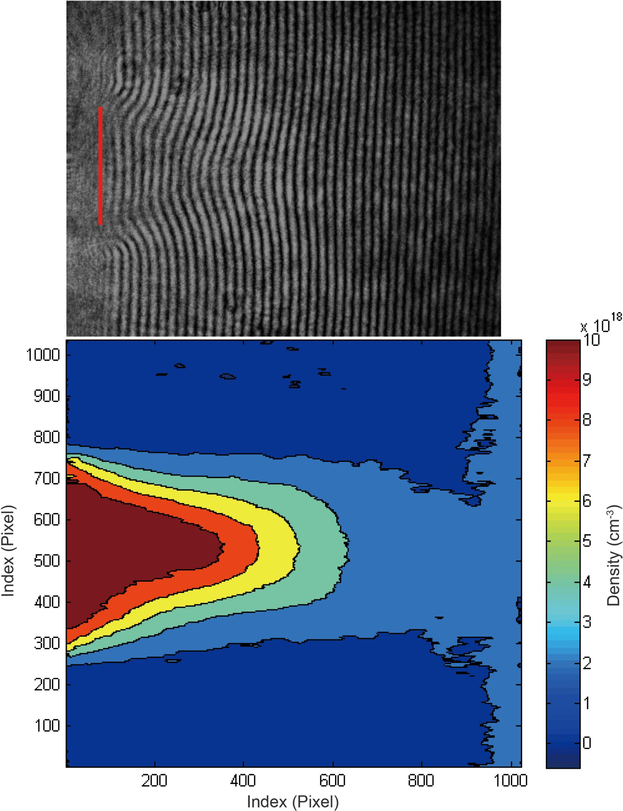
An interferometric measurement can be performed over a extended area of the plasma using an optical imaging system and camera as the light detector to acquire an image (the so-called interferogram), which enables 2D mapping of the line-integrated density over the light beam cross-section. In such a case, a numerical analysis of the interferogram is necessary to extract the actual phase shift using a phase-retrieval algorithm comprising phase-unwrapping procedures. Such measurements allow one to obtain an actual 2D map of the density, which is necessary to understand and monitor physical phenomena in ultra-fast laser–plasma interactions, especially during alignment and tuning of the LPA stages. As an example of a 2D measurement, in Figure 1 an interferogram of a supersonic gas jet in vacuum acquired by a Nomarski interferometer is shown, along with the density map retrieved from a phase-retrieval algorithm. Conversely, a 1D measurement of the average density along the laser beam path in the sample is performed when the intensity over the entire light beam cross-section is acquired using a photodiode or a photomultiplier tube (PMT) as the light detector. These 1D measurements are much faster and require less intense data analysis than the 2D measurements, making them potentially more suitable during LPA operation (for example, to monitor in real time the particle number density in the interaction region).

The main interferometric methods used to measure the particle density in LPA targets are schematically summarized in Figure 2 and discussed in the following.

In a two-arm interferometer (TAI) the phase shift is measured relative to the phase of a reference optical beam not passing through the sample but typically through a vacuum where the refractive index value is unity. The measured phase shift is then given by $\unicode[STIX]{x0394}\unicode[STIX]{x1D719}_{\text{TAI}}(\unicode[STIX]{x1D706})=\frac{2\unicode[STIX]{x03C0}}{\unicode[STIX]{x1D706}}\int _{L}[\unicode[STIX]{x1D702}(\unicode[STIX]{x1D706})-1]\,\text{d}l$. Two-arm interferometry can be implemented in two main configurations, depending on the optical design adopted.

Standard TAI, such as Mach–Zehnder interferometers, where the light beam is split into two distinct beams following different geometrical paths, called the reference and measurement arms, which are then recombined and interfere^{[7, 23, 24]}.Modified TAIs, also called two-arm folded, where the light beam is split into two parts after passing through the sample, and interference takes place between the part of the beam that has passed through the sample and the part of the beam not passing through the sample^{[18, 25]}. This method provides good control on the fringe spacing and image formation.

The standard TAIs suffer from a very high susceptibility to environmental conditions (for example, mechanical vibration and temperature changes) while the folded TAI is relatively more robust against environmental conditions due to the more compact size of the two-arm section. The typical sensitivity of an ultra-fast imaging TAI can be hundredths of a fringe (${\sim}$0.1 rad). To achieve better sensitivity, on the order of a few millradians, special care has to be taken during the measurement by making use of a probe beam with very good quality, active mechanical stabilization and averaging^[19]. The latter may hamper implementation of TAIs for real-time measurement and online monitoring applications. However, TAIs may find applications for the characterization, alignment and optimization of LPA stages due to their versatility.

Besides time-domain measurements, also spectral-domain interferometry has been implemented in TAIs for the measurement of the free-electron density in discharged capillaries using ultra-fast laser pulses^{[26, 27]}. These measurements are based on the density-dependent group velocity of an ultra-short laser pulse when propagating in a plasma channel^[13]. Specifically, the group velocity delay between a laser pulse propagating in vacuum and a laser pulse propagating through the plasma inside the discharged capillary actually depends on the mismatch of the group index of refraction due to the free electrons. However, such a two-arm configuration poses serious challenges which prevent its use in monitoring discharged capillary-based LPA for high-quality accelerators in user-oriented facilities. This limitation can be overcome by instead adopting spectral-domain second-harmonic interferometry, as will be discussed later.

These are similar in principle to the modified TAI, and the phase measured is exactly the same (reference beam in vacuum and signal beam over the object), but they have a somewhat easier setup, being a quasi-common-path configuration with minimal geometrical separation between the two interfering parts of the beam. Typical configurations are as follows.

Standard Nomarski interferometer, where the two interfering beams are separated by means of a Wollaston beam splitter and interference is recorded after a polarizer^[28–30].Fresnel bi-prism interferometer, which is based on the use of a Fresnel bi-prism that allows one to overlap directly two different parts of the same input beam^[31].

A versatile and robust method to measure phase variations across a light beam is based on the use of wavefront (WF) sensors (for example, the quadri-wave lateral shearing interferometer^[32]). This instrument measures the phase difference between two adjacent points of the light beam cross-section by means of a wavefront detector. In fact this method is sensitive to phase gradients of the beam cross-section along two orthogonal directions, and the actual 2D map of the phase is retrieved by analyzing the data with specific software. Finally, the phase shift of interest is calculated by subtracting the phase map of an undisturbed beam acquired in a separate measurement without the sample^[33]. It can be considered a single-arm configuration, since interference takes place only at the detector, and is therefore a very robust method allowing for easy installation with a phase sensitivity which is stated to be ${<}$2 nm (that is, ${<}$30 mrad at 400 nm)^[34]. A value of 11 mrad has actually been estimated as the root-mean-square over 188 acquisitions using 400 nm laser light^[35]. It must be noted that a single-acquisition value has not been reported to our best knowledge, so a conservative value of 30 mrad at 400 nm is assumed here.

Of note, the wavefront of a laser beam, and the density information contained therein, can be extracted also by numerical beam intensity analysis of standard 2D images from a camera, with a phase resolution of about 80 mrad^[36]. However, the numerical analysis involves multiple images for this approach to be effective, thus limiting its applicability for real-time measurements, but it could be suitable for offline tuning and optimization of LPA stages.

Another kind of interferometric approach for the measurement of particle density in optically dispersive samples (for example, neutral gas or plasma) is based on the so-called second-harmonic interferometer (SHI), also known as the dispersion interferometer. The SHI has a fully common-path configuration and is sensitive to the phase difference acquired by the fundamental and second-harmonic beams when passing collinearly through the sample^{[37, 38]}. The measured phase shift is given by $\unicode[STIX]{x0394}\unicode[STIX]{x1D719}_{\text{SHI}}=\frac{4\unicode[STIX]{x1D70B}}{\unicode[STIX]{x1D706}}\int _{L}\unicode[STIX]{x0394}\unicode[STIX]{x1D702}(l,\unicode[STIX]{x1D706})\,\text{d}l=\frac{4\unicode[STIX]{x1D70B}}{\unicode[STIX]{x1D706}}L\overline{\unicode[STIX]{x1D6E5}\unicode[STIX]{x1D702}}(\unicode[STIX]{x1D706})$, where $\unicode[STIX]{x0394}\unicode[STIX]{x1D702}(\unicode[STIX]{x1D706})=\unicode[STIX]{x1D702}(\unicode[STIX]{x1D706})-\unicode[STIX]{x1D702}(\unicode[STIX]{x1D706}/2)$. It is a very robust method against mechanical vibrations and environmental conditions in general, and it can reach a phase sensitivity of less then 1 mrad for 1D measurements without requiring any vibration mitigation system^[39]. Although 2D measurements using the SHI method have been demonstrated^{[40, 41]}, there is no quantitative data available in the literature regarding the sensitivity of the imaging SHI. Here, we assume a conservative value of 10 mrad for quadrature detection^{[39, 42]}. To date, SHIs have mostly been developed and applied to monitor the free-electron density in magnetically confined large plasma machines^{[43, 44]}. Recently, due to their versatility and robustness, SHIs have been successfully applied also for the characterization and monitoring of gas targets for LWFA (namely discharged gas-filled capillaries^{[45, 46]} and gas cells^{[21, 47]}).

Specifically, spectral-domain (SD) second-harmonic interferometry^[48] has been adopted instead of spectral-domain TAI to monitor the density inside a discharged gas-filled capillary, due to the much easier implementation and much higher stability of the common-path configuration compared to the two-arm design^[45]. In an SD SHI, the spectral interference takes place between the second-harmonic pulse generated before the sample and the time-delayed second-harmonic pulse generated after the fundamental pulse has propagated through the sample. The time delay $\unicode[STIX]{x0394}T$ between the two second-harmonic ultra-short pulses arises from the different group velocities in the sample at the fundamental and second-harmonic wavelengths, which is proportional to the density. In terms of phase, the pulse envelope slippage due to the plasma is $\frac{4\unicode[STIX]{x1D70B}}{\unicode[STIX]{x1D706}}c\unicode[STIX]{x0394}T$, where $\unicode[STIX]{x1D706}$ is the fundamental laser wavelength. The time delay is estimated by measuring the modulation period $\unicode[STIX]{x0394}\unicode[STIX]{x1D708}$ in the frequency spectrum of the two interfering pulses ($\unicode[STIX]{x0394}T=1/\unicode[STIX]{x0394}\unicode[STIX]{x1D708}$). For laser pulses propagating in a discharged gas-filled capillary with a near-match guided configuration typical for LPA, the relation between the time delay $\unicode[STIX]{x0394}T$ and the average on-axis plasma density $n_{e}$ can be approximated very well by assuming free propagation in a plasma with an average density $n_{e}$^[45], resulting in the same phase shift as a function of the electron density (see Table 1). When applying SD interferometry, also the spectral phase of the modulated frequency spectrum can be measured. It is noted that, given a linear response of the plasma, the phase shift due to the different group velocities (group delay) and the phase shift due to the different phase velocities (spectral phase shift) have the same magnitude but opposite sign. Recently, sensitivities of 2.85 rad in group-delay measurements and of 63 mrad for spectral phase measurements have been demonstrated^[46].

The use of a continuous-wave (CW) laser-based SHI has been successfully demonstrated for high-resolution real-time monitoring of the gas density inside a gas flow cell placed in a vacuum chamber^{[21, 47]}. As an example, Figure 3 reports the results of real-time measurements by a CW 1064 nm second-harmonic interferometer of the Ar gas number density inside a pulsed gas flow cell specifically developed for LWFA (SourceLAB, Model SL-ALC). The measurement is performed transversely over a length of 35 mm for a backing pressure of 600 mbar (1 bar $=$ 100 kPa) and for gas pulse lengths of 100 ms and 500 ms.

A specific issue common to all time-domain interferometric measurements is related to the periodic evolution of the intensity pattern with alternating minima and maxima in the detected light intensity, which gives rise to so-called fringes. This fact implies that measurements of a phase shift that spans multiple fringes may become indeterminate when retrieving the absolute phase shift from the measured intensity data. Typically, this issue is addressed during the data analysis with specific phase-unwrapping protocols. There are two basic requirements for such phase-unwrapping protocols to be effective. First, the presence of a reference data point with known phase shift, typically zero, with respect to which all other phase shifts are referred. In 2D measurements such data can be a pixel or an area of the image where the two interfering beams have the exact same phase, while in 1D measurements the reference value is typically obtained from the data acquired before the event under investigation has started or by waiting until its completion. Second, the measurements have to resolve all fringes. In 2D measurements this means that the spatial gradient of the phase to be measured must be small enough to avoid fringe jumps between two adjacent pixels of the detector^[49]. In 1D measurements, the detector has to be fast enough to accurately follow the evolution in time of the interference signal in order to count the number of fringes^[50].

When the measured phase shift is small enough to stay within a half-fringe so that it can be determined unambiguously, i.e., $\unicode[STIX]{x0394}\unicode[STIX]{x1D719}<\unicode[STIX]{x1D70B}$, then fringe jumps are avoided and phase-tracking or phase-unwrapping protocols are not necessary, enhancing the phase measurement sensitivity and speed, and allowing for more robust real-time monitoring. As an example, the maximum density shown in Figure 3 corresponds to approximately 0.5 bar pressure at room temperature, which would result in a ${\sim}27$  rad phase shift (${>}$4 fringes) in a TAI^[51], while the phase shift read by the SHI is ${<}1$  rad^[52], thus sub-fringe, allowing for a real-time measurement.

It is highlighted that a time delay measurement in SD interferometry is inherently immune to the fringe-jump issue, and can be applied to measure plasma densities over relatively long distances, which would result in a signal spanning many fringes in a time-domain measurement. As an example, when adopting SD second-harmonic interferometry to measure the electron density in gas discharged capillary^[46] the group-delay measurement is used to determine the number of fringes, thanks to a sub-fringe phase resolution of 2.85 rad, while the simultaneous determination of the spectral phase allows one to achieve an overall 63 mrad phase resolution over multiple fringes.

The actual relation between the measured phase shift and the particle density is different in the case of neutral particles in a gas or free electrons in a plasma. The values of the refractivity of hydrogen at STP for the fundamental and second-harmonic wavelengths of a Ti:sapphire laser are $\unicode[STIX]{x1D702}(800)=1.374\times 10^{-4}$ and $\unicode[STIX]{x1D702}(400)=1.426\times 10^{-4}$, respectively^[53], thus $\unicode[STIX]{x0394}\unicode[STIX]{x1D702}(800)=\unicode[STIX]{x1D702}(400)-\unicode[STIX]{x1D702}(800)=52\times 10^{-7}$. So, based on these values and on the known equation for the plasma refractive index as a function of wavelength and electron density, the expected phase shifts can be evaluated and are reported in Table 1. The wavelength reported for SHI is the fundamental wavelength used, while the reported phase refers to the detected second harmonic, i.e., 400 nm wavelength. It is noted that the phase to be measured by Nomarski-type interferometers is actually the same as for the TAI.

The wavefront sensor measures only the gradient of the density, and therefore there is no straightforward analytical relation between the measured quantity and the density which is determined from the phase extracted by dedicated software. A comparison between similar measurements performed with both wavefront-based sensors and a modified TAI revealed a difference in the absolute value of the measured density of 10%–20%^[35]. Indeed, a 15 nm accuracy is stated for the instrument^[34], i.e., 0.24 rad at 400 nm, which can explain the deviation of the absolute value found with respect to the modified TAI measurement. Thus, the WF-sensor-based instrument requires an accurate calibration before being used for the absolute measurement of density. For comparison, the SHI employing quadrature detection can reach an absolute accuracy of 1% or less for 1D measurements^[39].

In Figures 4 and 5 the capabilities of the various interferometric methods are shown graphically for neutral hydrogen and free electrons, respectively: the full lines represent the lower detection limit set by the sensitivity, while the dashed lines represent the upper limit for measurement within a single fringe, i.e., $\unicode[STIX]{x0394}\unicode[STIX]{x1D719}<\unicode[STIX]{x1D70B}$. Of course a fringe jump allows one to overcome this upper limit, but at the expense of higher uncertainty in time-domain measurements. As discussed, fringe jumps are not an issue in spectral-domain interferometry, thanks to simultaneous group-delay and spectral phase measurements. In Figure 5 the capabilities in terms of the phase of both group-delay and spectral phase measurements are reported separately.

Interferometry is usually performed transversely to the main laser beam. In such a case, the plasma length covered by the interferometer light beam lies between $10~\unicode[STIX]{x03BC}\text{m}$ (roughly the dimensions of the main laser beam spot) and hundreds of $\unicode[STIX]{x03BC}\text{m}$. The transverse neutral gas length can range from ${\sim}$mm typical for pulsed jets^[17] to tens of millimeters in gas flow cells^{[21, 24, 54]}.

For neutral hydrogen measurements, from Figure 4 it is evident that both the SHI and the WF-based sensors are capable of measuring low density values, even for few millimeters path. The 1D measurement with the SHI allows very fast monitoring of the neutral hydrogen density (acquisition time ${\sim}1~\unicode[STIX]{x03BC}\text{s}$) and can be implemented as a sensor in closed-loop gas flow regulation systems. This is very important when gas cells are used. In fact, repetitive shots of the high-power main laser beam will eventually modify the cell’s orifice, usually of hundreds of microns diameter, altering the gas flow dynamics and therefore the actual gas number density inside the cell for a pre-set backing pressure^[12]. Online regulation of such a gas supply system is therefore necessary in order to achieve a stable and reproducible laser-plasma acceleration process. The 1D measurement with the SHI can achieve a sensitivity of ${<}$1 mrad, therefore enabling the measurement of densities of about $10^{17}~\text{cm}^{-3}$ over a 1 mm length^[39]. The WF sensor is indeed suitable for 2D mapping, starting at a few $10^{17}~\text{cm}^{-3}$ and few millimeters in length. As per the higher values of density and medium length, all the methods can measure within a single fringe for millimeter-sized sample with densities up to $10^{19}~\text{cm}^{-3}$, except the TAI interferometer at 400 nm.

For free-electron density measurements, Figure 5 shows that only the imaging SHI with 10 mrad sensitivity would be suitable to measure the lowest free-electron density in the range of few $10^{17}~\text{cm}^{-3}$ for a plasma length ${<}100~\unicode[STIX]{x03BC}\text{m}$. However, such an instrument has not been tested yet and further development is necessary to assess the actual sensitivity achievable with the imaging SHI. An ultra-fast probe beam has to be used to monitor the free electrons during laser–plasma interactions. Ultra-fast SHI has been presented in the literature^{[42, 55]}, but more development is necessary to establish a femtosecond version of the SHI. The WF-sensor-based instrument is suitable for the measurement of free-electron densities ${>}10^{18}~\text{cm}^{-3}$ with plasma paths longer than hundreds of $\unicode[STIX]{x03BC}\text{m}$, and it can work readily with ultra-fast light sources^[35]. In Figure 5 the capability of SD second-harmonic interferometry is also reported. High-sensitivity spectral phase measurements, combined with group-delay measurements over multiple fringes, are ideal candidates as diagnostics to monitor the electron density inside gas discharged capillaries with relatively large line-integrated densities.

The advantages and disadvantages (pros and cons) of each interferometric method are summarized in Table 2.

All interferometric methods require an appropriate optical line of sight through the sample. In the case of a freely expanding gas jet, interferometry is easy to implement, whereas in the case of confined samples (for example, gas cells, capillaries and tubes), flat optical side windows are necessary to provide the optical path for transverse interferometry. This issue must be considered when designing the actual geometry of the accelerator stage. When a straight optical path through the sample is not available (for example, cylindrical capillary or tubes) optical emission spectroscopy can be considered as a means to monitor the density. Specifically, Stark broadening of hydrogen emission lines and wavelength-shifted Raman scattering of the main laser beam will be considered here.

Spectroscopic investigation of hydrogen emission lines (for example, $\text{H}_{\unicode[STIX]{x1D6FC}}$ at 656.3 nm and $\text{H}_{\unicode[STIX]{x1D6FD}}$ at 486.1 nm) may be implemented to monitor the free electron density with a relatively simple approach^[56]. In fact, the electron density can be estimated from the broadening of the hydrogen emission lines as $$\begin{eqnarray}n_{e}=8.02\times 10^{12}(\unicode[STIX]{x0394}\unicode[STIX]{x1D706}_{1/2}/\unicode[STIX]{x1D6FC}_{1/2})^{3/2},\end{eqnarray}$$ (1) where $n_{e}$ is in $\text{cm}^{-3}$ and $\unicode[STIX]{x0394}\unicode[STIX]{x1D706}_{1/2}$, the full width at half-maximum of the Stark-broadened spectral line, in ångstroms. The data analysis in this case depends (slightly) on the actual electron temperature via the tabulated parameter $\unicode[STIX]{x1D6FC}_{1/2}$^[56], and therefore a measurement (or at least a reliable estimate) of the electron temperature may be necessary in parallel with Stark broadening measurements. Remarkably, the plasma temperature can be estimated from the spectroscopic measurement via the ratio of the emission line to the background underlying continuum^{[57, 58]}. Stark broadening measurements can be performed both longitudinally^[59–63] and transversely^{[9, 64, 65]}, as shown schematically in Figure 6. Spatially resolved emission spectroscopy can be implemented using an imaging spectrometer, and measurements on the nanosecond time scale can be achieved using a fast camera^[66]. For example, Stark broadening of $\text{H}_{\unicode[STIX]{x1D6FD}}$ allows the local electron density with values ${<}10^{17}~\text{cm}^{-3}$ to be determined with a medium-resolution spectrometer. An experimental study comparing transverse TAI and longitudinal Stark broadening measurements of $\text{H}_{\unicode[STIX]{x1D6FD}}$^[63] has demonstrated very good agreement between the two measurement methods.

Measurement of the Raman scattering of the main laser beam photons due to the plasma can give information on the local free-electron density^[67]. In fact, the frequency of the Raman scattered signal $\unicode[STIX]{x1D714}_{R}$ is shifted compared to the original laser frequency, $\unicode[STIX]{x1D714}_{L}$ by the plasma frequency $\unicode[STIX]{x1D714}_{p}$, i.e., $\unicode[STIX]{x1D714}_{R}=\unicode[STIX]{x1D714}_{L}-\unicode[STIX]{x1D714}_{p}$, so that the free-electron density can be estimated as $$\begin{eqnarray}n_{e}=1.11\times 10^{8}(1/\unicode[STIX]{x1D706}_{L}-1/\unicode[STIX]{x1D706}_{R})^{2},\end{eqnarray}$$ (2) where $n_{e}$ is expressed in $10^{19}~\text{cm}^{-3}$ and the wavelength in nanometers^[68]. Raman scattering can be measured in the forward or backward directions compared to the main laser beam, as schematically shown in Figure 7. The implementation of forward scattering measurements in LWFA experiments requires the use of a mirror with a hole in the center such that the Raman radiation is reflected while the electron bunch can propagate undisturbed^[69], whereas the backward measurement can be performed mainly at wavelengths outside the reflectivity range of the main laser beam mirror^[70].

An experimental study comparing the free-electron density inside a 15-mm-long discharged gas-filled capillary measured by TAI and estimated by the frequency shift between the original TW level main laser wavelength and the forward-scattered Raman light has indicated a good agreement between the two diagnostics up to $10^{19}~\text{cm}^{-3}$^[69]. However, strong discrepancies in the Raman-based measurement can occur above $10^{19}~\text{cm}^{-3}$^[70]. On the other hand, densities ${<}10^{18}~\text{cm}^{-3}$ are difficult to quantify by this methodology since the wavelength shift and the scattered light intensity may be too low to be accurately measured, due also to the spurious light from the high-intensity main laser beam. So, this methodology is indeed interesting for high-quality LPA due to its relatively simple implementation, but would be useful mainly for free-electron densities in the range $10^{18}$–$10^{19}~\text{cm}^{-3}$.

Besides forward and backward Raman scattering, it is worth noting that the measurement of side Raman scattering of the main laser pulse interacting with the plasma can also provide a monitor of the electron number density^[71]. A systematic experimental investigation of the spatial–spectral properties of the side emission scattered out of the polarization plane of the drive intense laser pulse during LWFA has shown a correlation between the wavelength shift of the Stokes line of Raman side scattering and the electron number density^[72]. In the specific case, a detailed analysis of the recorded spectral shifts as a function of the electron number density, measured independently by interferometry in the range $10^{18}{-}10^{19}~\text{cm}^{-3}$, revealed a very good agreement with relativistic stimulated Raman scattering theory in plasmas at a high laser intensity, demonstrating the feasibility of Raman side scattering measurements as a density diagnostic tool. From a practical point of view, side Raman scattering measurements, being somehow easier to implement than forward and backward scattering measurements, could provide an online monitor of the accelerator performance as well as a density monitor during alignment, optimization and operation of an LPA once it is calibrated by means of other methodologies (for example, interferometry).

For LPA stages in the range 0.1–1 GeV (for example, injector in multi-stage systems) the corresponding electron density is in the range from a few $10^{17}~\text{cm}^{-3}$ up to a few $10^{18}~\text{cm}^{-3}$ (lower density $\rightarrow$ higher energy), and target configuration may be mm-long gas jets or gas flow cells. The 2D SHI potentially has the capability of accurate diagnostics for the electron density in the low density range, but further development is necessary to validate the ultra-fast and 2D imaging configuration. At higher density and/or greater plasma lengths the WF-sensor-based instrument provides a good solution for 2D mapping with ultra-fast resolution. Concerning neutral gas density measurements in the range $10^{17}{-}10^{19}~\text{cm}^{-3}$, 1D SHI provides a ready solution for real-time monitoring, while the WF sensor is suitable for 2D mapping.

For LPA stage(s) requiring greater acceleration lengths to reach electron energies of several GeV, plasma channels with densities in the range $10^{17}{-}10^{19}~\text{cm}^{-3}$ provide adequate target structures. In this context, small-diameter plasma channels created with a laser pre-pulse in gas cells are open structures that can allow transverse interferometry: at lower density only the ultra-fast 2D SHI may be useful, while at higher density the WF-sensor-based instrument may be adequate. However, this LPA configuration is difficult to control, involving two separate laser beams, and may pose serious challenges when adopted in user-oriented high-quality accelerators.

Concerning plasma channels created by a discharge in a capillary, they do not allow for transverse interferometry unless a square capillary cross-section is used. Then, Stark broadening/Raman scattering measurements and/or longitudinal interferometry may be adopted. Significantly, spectral-domain second-harmonic interferometry has recently been demonstrated to be an elegant and suitable methodology to monitor discharged gas-filled capillaries longitudinally. Combining simultaneous group-delay and spectral phase measurements, a high phase resolution has been achieved in measurements spanning multiple fringes.

TAI interferometers are in general less suitable for implementation during operation and they may be more useful during alignment/tuning of the system due to their well-established use in research laboratories.