Hyperspectral Image Classification via Multiple-Feature-Based Improved Sparse Representation

Feiyan Li; Hongtao Huo; Jing Li; Jie Bai

doi:10.3788/AOS201939.0528004

Journals >Acta Optica Sinica >Volume 39 >Issue 5 >Page 0528004 > Article

Acta Optica Sinica
Vol. 39, Issue 5, 0528004 (2019)

Hyperspectral Image Classification via Multiple-Feature-Based Improved Sparse Representation

Feiyan Li, Hongtao Huo^*, Jing Li, and Jie Bai

Author Affiliations

Information Technology and Cyber Security Academy, People's Public Security University of China, Beijing 100038, China

show less

DOI: 10.3788/AOS201939.0528004 Cite this Article Set citation alerts

Feiyan Li, Hongtao Huo, Jing Li, Jie Bai. Hyperspectral Image Classification via Multiple-Feature-Based Improved Sparse Representation[J]. Acta Optica Sinica, 2019, 39(5): 0528004 Copy Citation Text

show less

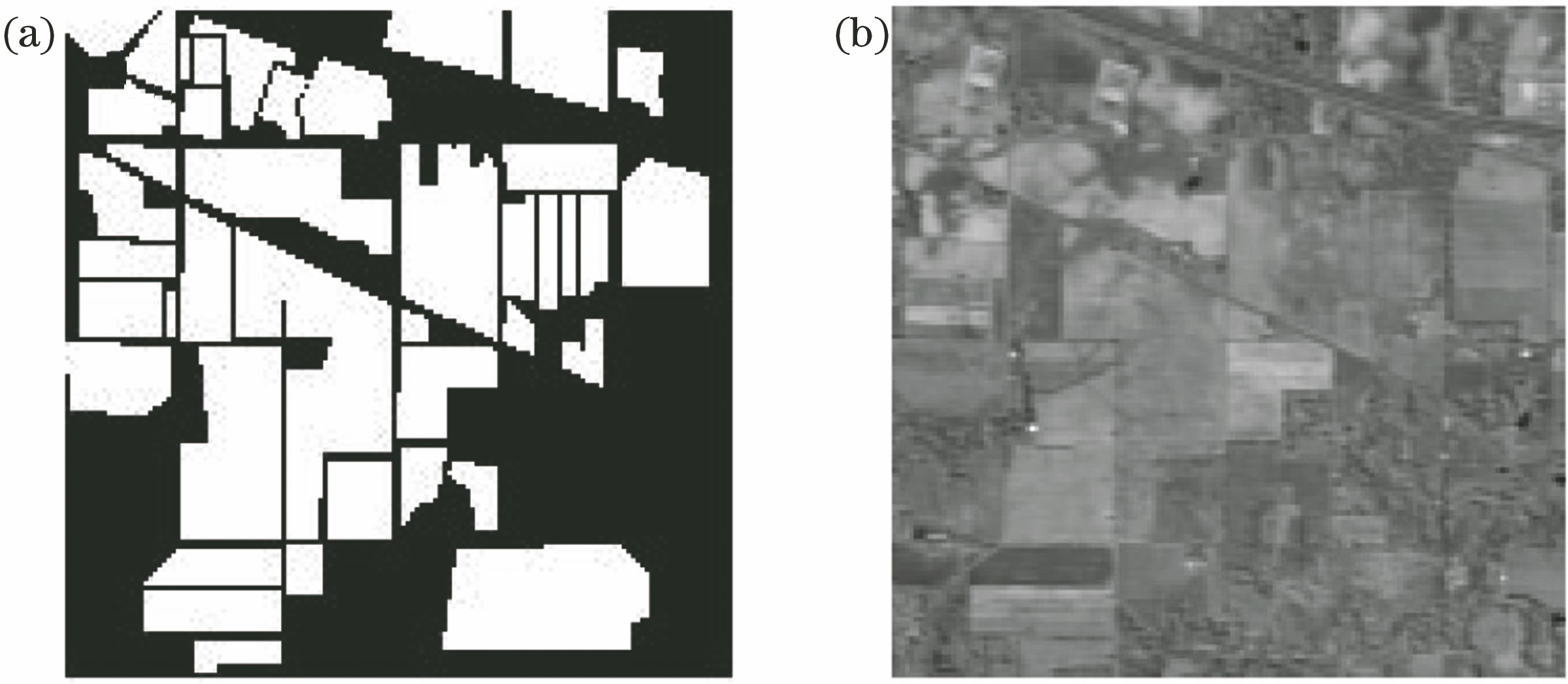
Fig. 1. Results of different feature extraction methods. (a) LBP; (b) Gabor

Download full size

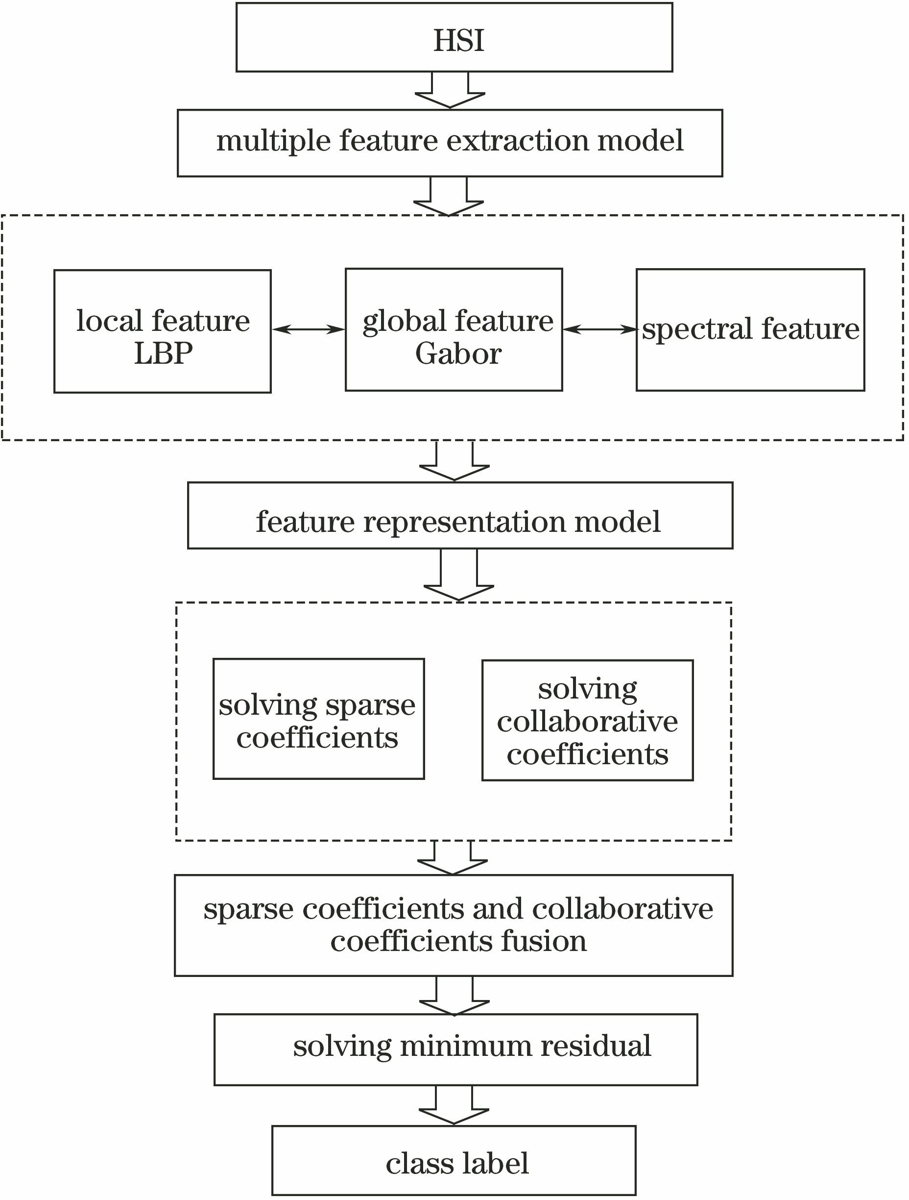
Fig. 2. Flow chart of MFISR

Download full size

Fig. 3. Parameter adjustment and accuracy change

Download full size

Fig. 4. Images of Salinas. (a) Pseudo-color image; (b) ground truth image

Download full size

Fig. 5. Classification maps of different methods on Salinas dataset. (a) SVM; (b) SRC_Spectral; (c) SRC_Gabor; (d) SRC_LBP; (e) CRC_Spectral; (f) CRC_Gabor; (g) CRC_LBP; (h) MFISR

Download full size

Fig. 6. Image of Indian Pines. (a) Pseudo-color image; (b) ground truth image

Download full size

Fig. 7. Classification maps of different methods on Indian Pines dataset. (a) SVM; (b) SRC_Spectral; (c) SRC_Gabor; (d) SRC_LBP; (e) CRC_Spectral; (f) CRC_Gabor; (g) CRC_LBP; (h) MFISR

Download full size

No.	Class	Training	Test
1	Brocoli_green_weeds_1	41	1968
2	Brocoli_green_weeds_2	75	3651
3	Fallow	40	1936
4	Fallow_rough_plow	28	1366
5	Fallow_smooth	54	2624
6	Stubble	80	3879
7	Celery	72	3507
8	Grapes_untrained	226	11045
9	Soil_vinyard_develop	125	6078
10	Corn_senesced_green_weeds	66	3212
11	Lettuce_romaine_4wk	22	1046
12	Lettuce_romaine_5wk	39	1888
13	Lettuce_romaine_6wk	19	897
14	Lettuce_romaine_7wk	22	1048
15	Vinyard_untrained	146	7122
16	Vinyard_vertical_trellis	37	1770
Total		1092	53037

Table 1. Training and test sample distributions of different class labels in Salinas dataset

No.	SVM	SRC_Spectral	SRC_Gabor	SRC_LBP	CRC_Spectral	CRC_Gabor	CRD_LBP	MFISR (Spectral Value+Gabor+LBP)
1	0.9563	0.8301	1	1	0.9918	0.9969	1	1
2	0.9726	0.9945	0.9978	0.9997	0.9703	0.9817	0.9989	1
3	0.8657	0.9770	0.9847	0.9938	0.9890	1	0.9954	1
4	0.9810	0.9941	0.9770	0.9020	0	0	0.8713	0.9109
5	0.9501	0.9926	0.9908	0.9767	0.5407	0.5306	0.9778	0.9519
6	0.9773	0.9943	0.9985	0.9922	0.9852	0.9888	0.9891	0.9809
7	0.9855	0.9864	0.9909	0.9923	0.9211	0.9372	0.9872	0.9991
8	0.8050	0.7934	0.8096	0.9995	0.6332	0.6315	0.9954	0.9968
9	0.9595	0.9932	0.9869	0.9975	0.7095	0.6796	0.9984	1
10	0.7883	0.9535	0.9478	0.9900	0.8268	0.8792	0.9872	0.9981
11	0.8203	0.9894	0.9311	0.9715	0.9419	0.9509	0.9581	0.9839
12	0.9529	0.9661	0.9697	0.9700	0.9655	0.8923	0.9721	0.9951
13	0.9588	0.9601	0.9310	0.9404	0	0	0.9100	0.8967
14	0.8664	0.9632	0.9615	0.9561	0.5205	0.5219	0.9324	0.9538
15	0.4985	0.7433	0.7863	0.9960	0.7073	0.7551	0.9947	0.9942
16	0.8254	0.9886	0.9948	1	0.9994	1	1	1
OA	0.8462	0.9068	0.9206	0.9898	0.7532	0.7508	0.9860	0.9890
AA	0.8852	0.9450	0.9537	0.9799	0.7314	0.7341	0.9730	0.9788

Table 2. Classification accuracies of different methods on Salinas dataset

No.	Class	Training	Test
1	Alfalfa	5	41
2	Corn-notill	143	1285
3	Corn-mintill	83	747
4	Corn	24	213
5	Grass-pasture	49	434
6	Grass-trees	73	657
7	Grass-pasture-mowed	3	25
8	Hay-windrowed	48	430
9	Oats	2	18
10	Soybean-notill	97	875
11	Soybean-mintill	246	2209
12	Soybean-clean	60	533
13	Wheat	21	184
14	Woods	127	1138
15	Buildings-grass-trees-drives	39	347
16	Stone-steel-towers	10	83
Total		1030	9219

Table 3. Training and test sample distributions of different class labels in Indian Pines dataset

No.	SVM	SRC_Spectral	SRC_Gabor	SRC_LBP	CRC_Spectral	CRC_Gabor	CRC_LBP	MFISR (Spectral Value+Gabor+LBP)
1	0.7917	0.8947	0.9500	1	0	0	1	1
2	0.8070	0.8328	0.9030	0.9750	0.6468	0.6686	0.9641	0.9793
3	0.6720	0.8048	0.8643	0.9986	0.6352	0.7774	0.9901	0.9853
4	0.6381	0.6376	0.7828	0.9130	0	0	0.8787	1
5	0.8993	0.9486	0.9769	0.9824	0.9503	0.9932	0.9889	0.9823
6	0.9598	0.8997	0.9395	0.9985	0.7344	0.7616	0.9970	0.9868
7	0.8696	1	1	1	0	0	1	1
8	0.9705	0.9500	0.9731	1	0.8318	0.8286	1	1
9	0.4444	0.8333	0.9375	0.8500	0	0	0.9412	1
10	0.6693	0.8080	0.8801	1	0.7727	0.7857	0.9951	0.9783
11	0.7384	0.8366	0.9041	0.9955	0.5081	0.5436	0.9941	0.9933
12	0.7572	0.8505	0.9245	0.9768	0.8480	0.8532	0.9572	0.9835
13	0.9842	0.9643	0.9947	1	0.9895	1	1	1
14	0.9296	0.9269	0.9339	0.9915	0.8471	0.8691	0.9906	0.9890
15	0.6257	0.8354	0.8352	0.9688	0.9012	0.9524	0.9660	1
16	0.8824	0.9551	1	0.9412	0.9048	0.9710	0.9195	0.9753
OA	0.7957	0.8588	0.9115	0.9877	0.6593	0.6955	0.9825	0.9879
AA	0.7899	0.7997	0.8906	0.9652	0.7975	0.6253	0.9739	0.9908

Table 4. Classification accuracies of different methods on Indian Pines dataset

Feiyan Li, Hongtao Huo, Jing Li, Jie Bai. Hyperspectral Image Classification via Multiple-Feature-Based Improved Sparse Representation[J]. Acta Optica Sinica, 2019, 39(5): 0528004

Download Citation

Set citation alerts for the article

Tools

Set citation alerts for the article

Save the article for my favorites

Paper Information