With the development of the area of fast search and rescue for small and medium maritime targets for recent years， infrared target detection has been the main application method. Due to the complexity and change of the marine environment， it has brought certain difficulties to search and rescue targets. Therefore， it is necessary to classify the images of different scenes in order to improve the efficiency of target detection. It will facilitate subsequent image processing.

In recent years， image scene classification including natural scene and artificial scene is also an important research direction in the field of computer vision. The key to scene classification is image features extraction. Aiming at the extraction of image features， many classical methods have appeared， which are mainly divided into three categories ^［1］. One is a low-level method to extract feature descriptors directly from images， such as scale-invariant feature transform （SIFT）， color histogram and so on. The second is a mid-level method that continues feature extraction based on some underlying features of image block extraction， such as bag-of-visual-words （BOVW） and sparse coding. Thirdly， it is a high-level method to automatically extract features of images by training the network model of deep learning ^［2-3］.

Each of the three methods have advantages and disadvantages. The first method has simple steps， but the description of low-level features has limitations. Compared with the first method， the second method improves the classification accuracy， while the process is more complicated. Deep learning is a method emerging in recent years. The advantage is that the feature descriptors are not extracted manually， and well-trained network classification works very well. However， a large amount of data is required for training， which takes a long time and a high storage space.

In this paper， we use the low-level features because the whole process does not have much time and space in actual situations. And classification is performed by extracting the features of the sea background of the entire images， not sea targets. Common feature extraction methods of scene classification are SIFT， speeded-up robust feature （SURF）， local binary pattern （LBP）， HOG， and gray level co-occurrence matrix （GLCM） and so on.

Qilong Li et al. used SIFT algorithm to extract feature points， all feature points extracted are clustered by K-means clustering algorithm， and then bag of word （BOW） of each image is constructed. The SIFT algorithm has a strong tolerance for scaling， rotation， brightness changes， and noise ^［4］. Qiqi Zhu et al. proposed a local-global feature BOVW scene classifier for high spatial resolution imagery ^［5］. Atreyee Sinha et al. proposed a novel set of image descriptors. This image descriptor encoded information in image features and improves the popular directional gradient histogram pyramid （PHOG） descriptor for object and scene image classification ^［6］. Haitao Lang et al. used co-occurrence matrix to implant the spatial relations between local features， and proved that the feature co-occurrence matrix （FCM） is a potential discriminative character for scenes classification ^［7］.

At present， the infrared maritime target detection algorithms are relatively multiple and mature， but the background classification still has not received enough attention in the whole detection process. There is no single way to handle images with multiple situations. Therefore， it is necessary to study it carefully to improve the efficiency of search and rescue.

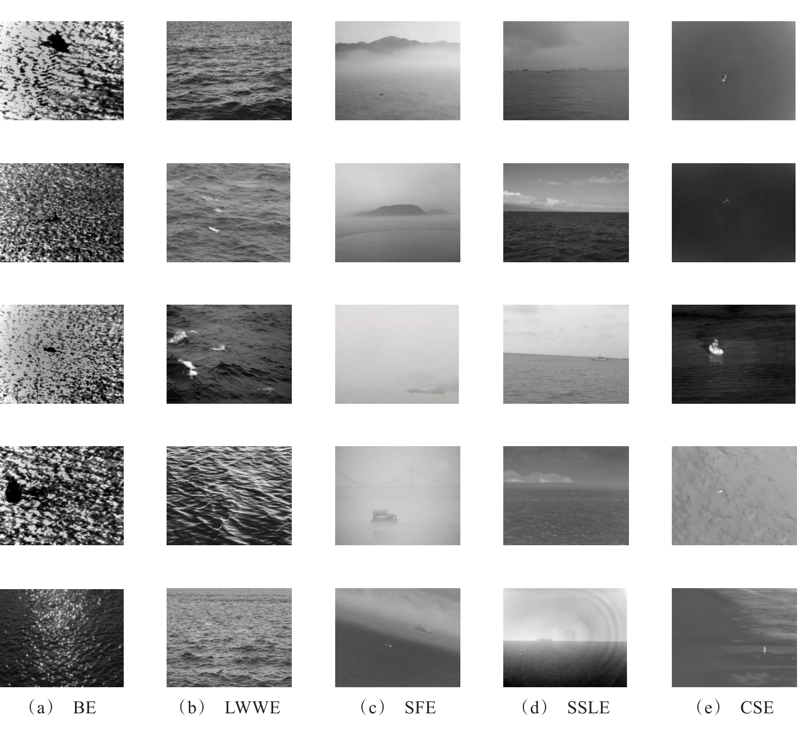
The sea background is complex and variable， and it will encounter various situations in the process of searching for targets， which may cause difficulty in target recognition and detection. Usually according to the actual needs of the sea rescue environment and target detection algorithms， marine background can be divided into five kinds of environment， namely， back-lighting environment （BE） ^［8］， large wind wave environment （LWWE） ^［9］， sea fog environment （SFE） ^［10］， sea-sky-line environment （SSLE） ^［11］， and calm sea environment （CSE）. Some images of each background are shown as Fig. 1. Gray distribution is shown in Fig. 2.

It can be seen from images that the overall brightness distribution of the BE image is uneven and has many spots. The background gray level of an image is unevenly distributed. LWWE texture information is irregular and clear， with stronger texture direction and weak correlation between gradients in different directions. The brightness distribution of the SFE image is not uniform. The difference between the foggy portion and the sea surface brightness is large， and the local background is smooth. The SSLE image is divided into sea surface part and sky part by sea-sky-line， including cloud， islands and so on. The sky part has high grayscale and clear texture information. Since images of different environments have different characteristics， they can be classified.

When multiple scenes appear in an image， we define the classification priority to these scenes. According to the actual situation， there are up to three situations. One is SSLE coexists with LWWE， one is both SSLE and BE exist simultaneously， and the other is both BE and LWWE exist side by side. The order for priority is SSLE， BE and LWWE. The image is shown as Fig. 3. It is classified as SSLE.

The targets include small and medium targets， mainly ships， and the application scenario is sea rescue search. Therefore， when the target exists in the background， the local characteristics of the background and the target position are less affected. There is no uniform influence rule， so the local features have less influence on global features. For the overall sea surface background， feature extraction is performed from two aspects.

The process of extraction of HOG and local contrast features are shown in Fig. 4. First， images are scaled to a uniform size （256*256 in this paper）， and the HOG features and local contrast are extracted respectively. The features are merged as shown as Fig. 5. Then a new feature vector is constructed and input into the classifier to complete an image classification task.

The content of feature extraction includes geometric or arithmetic descriptions of its color， grayscale， texture， contour， region， special point or line. Based on infrared imagery， it can be considered mainly from two aspects of texture and grayscale. Therefore， the HOG method and LCM are selected and combined to represent the characteristics of the image.

HOG is a feature descriptor used to describe local edge and shape information. It mainly calculates and counts the direction gradient histogram of the local region of the image. However， images of different backgrounds， such as SFE and SSLE， sometimes have similar grayscale distributions as shown in Fig. 6. Processing only the original image does not yield enough information， so dividing an image into a base layer and a detail layer allows for more comprehensive extraction of features such as Fig. 7. This paper uses Gaussian filtering to extract HOG features after layering the image. The size of the convolution kernel was determined to be 101 * 101 through multiple experiments， and σ = 20. Scan each pixel in the image in turn to perform a weighted average operation to obtain pixel values Q （x， y） at the corresponding position of the new image， which is a base image. Then a basic image is subtracted from an original image to obtain a detail image. Finally， the HOG feature of the whole image is obtained by tandem fusion.

The detailed process of extracting HOG features is as follows：

⋅ Step 1： Calculate the gradient and direction angle of each pixel of the image.

The gradient of the horizontal and vertical directions of the image pixels are calculated differently as follows：

Gx(x,y)=f(x+1,y+1)-f(x,y)

Gy(x,y)=f(x+1,y)-f(x,y+1)

In the above equation， represents pixel values， and represents the horizontal and vertical gradients at the pixel （x， y） in the input images. In this paper， the new one-dimensional central template operator is used to calculate the gradient values to reflecting local changes. Combined with the Robert operator， it is sensitive to curved edges. The gradient magnitude and gradient direction at the pixel （x， y） are as follows：

Gx,y=Gxx,y2+Gyx,y2

αx,y=tan-1Gyx,yGxx,y

The square root operation makes the process similar to what happens in the human visual system. The angle is divided into nine directions， and the corresponding gradient values are calculated respectively which are normalized as the feature vector of the gradient direction.

⋅ Step 2： Divide cell units and take the gradient direction histogram of each cell.

An image is divided into cells that each cell is 32*32 pixels， and the gradient information is counted by the histogram of 9 bins. The gradient size is used as the weight of the projection. It is obtained a 9-dimensional feature vector corresponding to the cell， that is， the gradient direction histogram of a cell.

If the size of the input image is 256 × 256， the small target will occupy less than 0.15% of it. This standard is usually independent of the size of the input image ^［12］. It is not necessary to extract more detailed features and reduce redundant information. Table 1 shows the comparison of different cell size under the same condition. It can be seen that small size takes a long time.

⋅ Step 3： Combine cell units into blocks and normalize gradient histograms within blocks.

Each cell is combined into a large， spatially connected interval， and the feature vectors of all cells in each block is concatenated and normalized to obtain the HOG feature of the block. The normalization method used is L2-Hys， which is obtained by first performing L2-norm， then clipping the result， and normalizing. L2-norm formula is setting as follows：

L2-norm:α=ββ22+e2

In this equation， β denotes a no normalized vector containing histogram information for a given block， e is a small constant， and the purpose is to avoid the denominator being 0； is the k-order norm of β.

⋅ Step 4： Get the HOG feature of the whole image.

The feature vectors of all the blocks in the detection window are concatenated to obtain the overall HOG feature vectors， which are combined into the final feature vector for classification.

Local contrast features are used to describe the grayscale variation of an image. Divided an image into blocks and analyzed the relationship between the central block and the surrounding blocks as shown in Fig. 8. And Fig. 9 shows the specific values of the matrix. An image is divided into n*n blocks， each block is composed of m*m pixels， and the maximum value and the average value of each block is calculated separately. Then each block is compared with the 8 surrounding blocks to form a 3*3 image window， which will slide sequentially to calculate the contrast of each block.

The local contrast is calculated as follows：

Cn=maxn(M0)meann(Mi)

In the equation， represents the contrast of nth image block， and indicates the maximum value of the nth block as the intermediate block， （i=1， 2， ...， 8） means the average of the surrounding blocks of the nth block.

The calculated values of each block form a 16*16 matrix， which is then arranged to obtain a one-dimensional feature vector of the entire image of 256×256 size. Fig. 10 calculates the local contrast of five different backgrounds. It can be seen that each category has different characteristics. The values of BE and LWWE fluctuate greatly， but they have no obvious rules of change. So， it is necessary to combine the HOG method mentioned above extracting more features. The values of SFE and SSLE have a trend from high to low that SSLE changes significantly from high to low and SFE is relatively flat. However， there is also a case where the difference in brightness between the sky and the sea surface is not obvious as shown in Fig. 8 SSLE-④. For example， Fig. 8 also shows the trend of SFE-⑤ and SSLE-⑤ which is less consistent with the normal law than the respective identical backgrounds. At this time， the simple local features are not sufficient to reflect the background difference. The value of CSE is generally lower and smoother. In general， local contrast can be distinguished under normal conditions by four categories. BE and LWWE are considered one type because it is difficult to distinguish between the two. Therefore， the features of an image are jointly extracted in combination with the HOG features above.

Through the learning algorithm， the support vector machine （SVM） can automatically find the support vector with good discrimination ability. The constructed classifier can maximize the class-to-class interval， so it has better adaptability and higher classification accuracy. Combined with the image classification of this experiment， it has a good classification effect.

Usually， “one vs. rest” or "pair-wise" strategy ^［13］ is used to solve multi-class SVM， and one-to-one model is used in experiments which is simplified into multiple binary classifiers （SVMs） for multi-class learning. The N categories are paired in pairs， and a total of classification tasks are performed. The test samples are input into classifiers to obtain results. The category with the smallest distance after comparison is the final result. Divided into 5 categories in the experiment， and N = 5 is substituted into a total of 10 classifiers. It is determined by calculating the Euclidean distance.

The linear support vector machine learning model is a separated hyperplane . This plane can be used to distinguish between positive and negative samples without error and the distance to the two types of samples are maximum. The discriminant model is calculated as follows.

f(ω)=signωTx+b

The linear support vector machine learning is to minimize the objective function and transform it into an optimization function for a n-dimensional input （i = 1， 2， ...， N） with labels as shown below. The first term is the loss function. The loss function is shown as follows. In the equation， the response range is y ∊ ｛-1，1｝， and 1 for the positive class， and -1 otherwise.

minω,b∑i=1NLyi,fxi+λ||ω||2

Lyi,fxi=max0,1-yifxii=1,2,…,N

Combined with the idea of the optimal classification straight line to be found， which is the straight line with the largest distance to the two types of class point sets， the objective function at this time can be abstracted：

maxω,bd=maxω,b1||ω||

minω,bω=minω,b12ωTω

The constraints satisfy the inequality constraint as follows.

yiωTx+b-1≥0i=1,2,…,N

Construct a Lagrange function， where is the Lagrangian coefficient， find the partial differential of ， and find the optimal classification function. represents the support vector， and represents the vector to be discriminated.

f(x)=signω*Tx+b*=sign∑i=1Nai*yi∅xi∅xj+b*

When the complexity of the data becomes large and cannot be separated linearly， the data is mapped into a high-dimensional feature space so that the data is linearly separable in the feature space. This mapping is denoted as . Since the inner product has a very large calculation dimension， a kernel function is introduced.

The number of samples in the experiment is 330 images， and the total feature dimension extracted is 3784. According to the prior knowledge of the experts， the ratio of the feature dimension to the number of samples is greater than 10， and usually a linear kernel function is used. The expression of the linear kernel function is as follows.

Kxi,xj=xiTxj

The inner product in the classification decision function can also be replaced by a kernel function， and the classification decision function becomes the form shown below.

f(x)=sign∑i=1Nai*yiKxi,xj+b*

This paper selects image captured by the actual shooting and qualified images found online. The data set consists of 5 categories. The training set contains 330 images， all of which are measured to 256*256 pixels in size. 250 images are kept for testing. Combining with SVM classifier， a one-to-one model is used for classification test. The operating environment is window7 operating system and the memory is 2G. The simulation platform uses matlab2016b version. The test was repeated 10 times， and the randomness was eliminated on average.

The results of using the new method are shown in the Table 2. There are 250 test images. Nine images were misclassified， and seven of them contained multiple scenes. It can be seen that the classification error rate of multiple types of backgrounds in the same frame of images accounts for 77.8% of the total misjudged images. Images containing multiple types of scenes are misjudged， such as Table 3. Multiple types of scenes are in the same image， including SSLE and SFE. However， the characteristics of SSLE are more obvious than those of SFE. It is easy to misclassify it by a classifier.

Some common feature extraction methods have been selected for comparison. Other methods for comparison with the new method include circular LBP（r=2， neighbor=8）， HOG， BOF， circular LBP（r=2，neighbor=8）+HOG ^［14］， Gaussian filter +HOG. The comparison of the correct rate and time of algorithms by many experimental data statistics is shown in Fig. 11. It can be seen that the accuracy of the improved feature is effective than the single feature extraction and the traditional combination methods. The accuracy of the new method reached 96.4%. At the same time， the method has good working performance in combination with accuracy and time cost.

This paper proposes an improved infrared images classification method based on improved features， which facilitates subsequent processing of different backgrounds and has practical significance. Combined with the new features， the infrared images of sea surface can be divided into 5 backgrounds. The image features are combined with the HOG feature extraction method of the improved extraction template and LCM. Under the same condition， the classification effect of the new features is better than that of single-use HOG features. At the same time， it is also compared with some common feature extraction methods. Experimental results show that this method has a good consequent to meet practice requirements.

References

[1] Gui-Song XIA, Jing-Wen HU, Fan HU et al. AID: A Benchmark Data Set for Performance Evaluation of Aerial Scene Classification. IEEE Transactions on Geoscience and Remote Sensing, 55, 3965-3981(2017).
[2] Jun CHU, Zhi-Xian GUO, Lu LENG. Object Detection Based on Multi-Layer Convolution Feature Fusion and Online Hard Example Mining. IEEE Access, 6, 19959-19967(2018).
[3] Yong-Mei REN, Jie YANG, Qing-Nian ZHANG, Zhi-Qiang GUO. Multi-Feature Fusion with Convolutional Neural Network for Ship Classification in Optical Images. Appl. Sci, 9, 4209(2019).
[4] Qi-Long LI, Xiao-Hong WANG. Image Classification Based on SIFT and SVM. 2018 IEEE/ACIS 17th International Conference on Computer and Information Science (ICIS)Singapore, 762-765(2018).
[5] Qi-Qi ZHU, Yan-Fei ZHONG, Bei ZHAO et al. Bag-of-Visual-Words Scene Classifier with Local and Global Features for High Spatial Resolution Remote Sensing Imagery. IEEE Geoscience and Remote Sensing Letters, 13, 747-751(2016).
[6] A. SINHA, S. BANERJI, Cheng-Jun LIU. New color GPHOG descriptors for object and scene image classification. Machine Vision and Applications, 25, 361-375(2014).
[7] Hai-Tao LANG, Yu-Yang XI, Jian-Ying HU et al. Scene Classification by Feature Co-occurrence Matrix. Computer Vision - ACCV 2014 Workshops, 501-510(2015).
[8] Li-Li DONG, Dong-Dong MA, Ge QIN et al. Infrared target detection in backlighting maritime environment based on visual attention model. Infrared Physics & Technology, 99, 193-200(2019).
[9] Song LI, Chun-Hua ZHANG, Min SHI. Neural network prediction model for ship hydraulic pressure signal under wind wave background. Journal of Shanghai Jiaotong University (Science), 2, 224-227(2015).
[10] Bin WANG, Li-Li DONG, Ming ZHAO et al. An infrared maritime target detection algorithm applicable to heavy sea fog. Infrared Physics & Technology, 71, 56-62(2015).
[11] Ying WEI, SHI Ze-Lin, Wavelet analysis. ISPA 2003. RomeItaly, 1, 23-28(2003).
[12] C. L. Philip Chen, Hong LI, Yan-Tao WEI et al. A Local Contrast Method for Small Infrared Target Detection. IEEE Transactions on Geoscience and Remote Sensing, 52, 574-581(2014).
[13] P Pratik. JOSHI, Randolph H. WYNNE, Valerie A. THOMAS. Cloud detection algorithm using SVM with SWIR2 and tasseled cap applied to Landsat 8. International Journal of Applied Earth Observation and Geoinformation, 82(2019).
[14] Guo-Long GAN, Jian CHENG. Pedestrian detection based on HOG-LBP feature. HainanChina, 1184(2011).
Set citation alerts for the article
Please enter your email address
© Copyright 2018-2021 | Chinese Laser Press. All Rights Reserved 沪ICP备15018463号-20