Comparative Analyses of Fitting Functions for Channel Impulse Response in Underwater Wireless Optical Communication Systems

Yueyue Tan; Yueheng Li; Ping Huang; Shanshan Liu; Meiyan Ju

doi:10.3788/AOS202141.1106001

Journals >Acta Optica Sinica >Volume 41 >Issue 11 >Page 1106001 > Article

Acta Optica Sinica
Vol. 41, Issue 11, 1106001 (2021)

Comparative Analyses of Fitting Functions for Channel Impulse Response in Underwater Wireless Optical Communication Systems

Yueyue Tan, Yueheng Li^*, Ping Huang, Shanshan Liu, and Meiyan Ju

Author Affiliations

School of Computer and Information, Hohai University, Nanjing, Jiangsu 211100, China

show less

DOI: 10.3788/AOS202141.1106001 Cite this Article Set citation alerts

Yueyue Tan, Yueheng Li, Ping Huang, Shanshan Liu, Meiyan Ju. Comparative Analyses of Fitting Functions for Channel Impulse Response in Underwater Wireless Optical Communication Systems[J]. Acta Optica Sinica, 2021, 41(11): 1106001 Copy Citation Text

show less

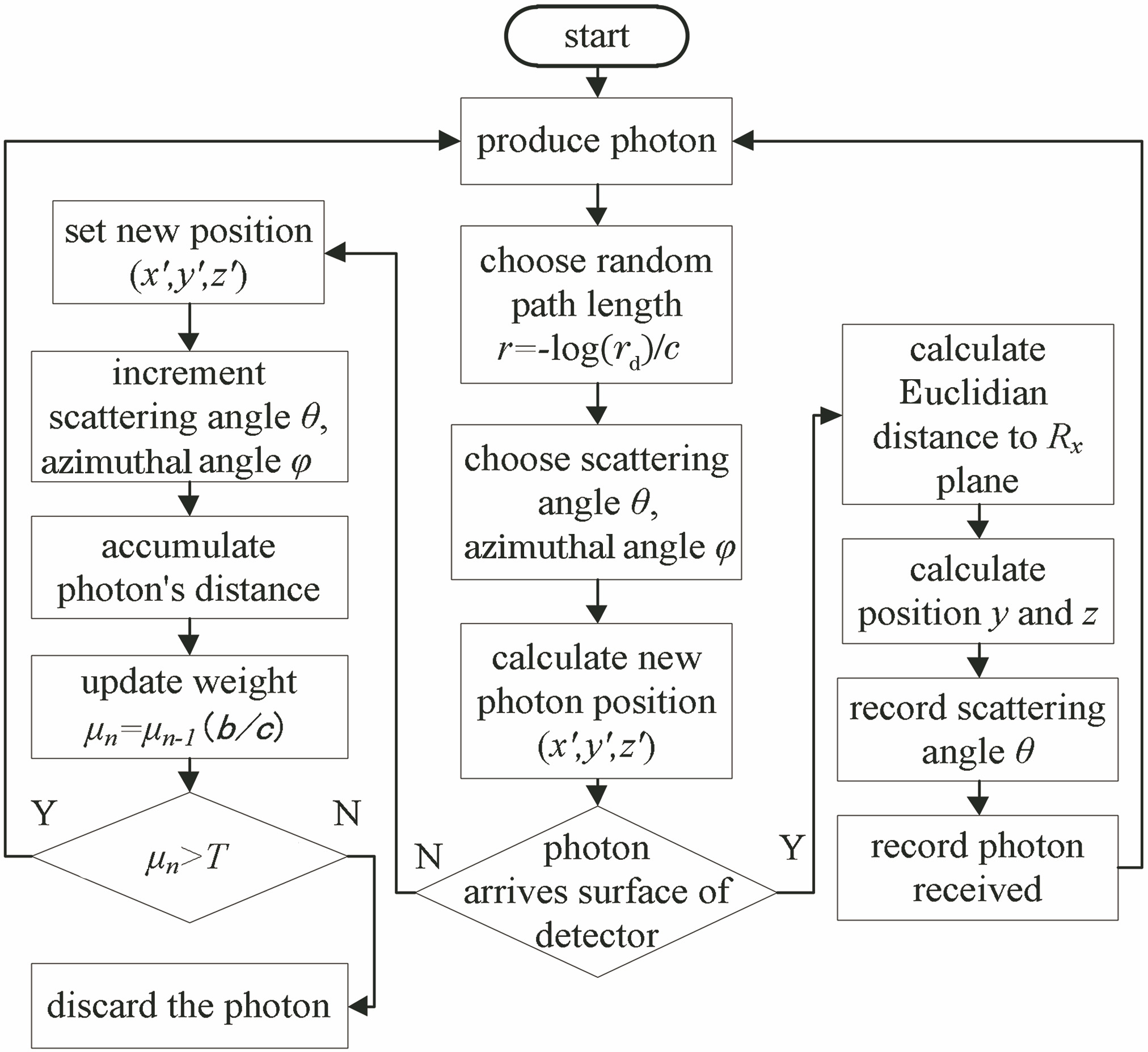
Fig. 1. Flowchart of Monte Carlo simulation in UWOC system

Download full size

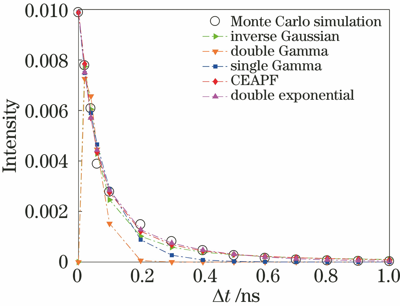
Fig. 2. Comparison between CIR curve simulated by Monte Carlo and various function fitting curves in clear ocean water

Download full size

Fig. 3. Comparison between CIR curve simulated by Monte Carlo and various function fitting curves in coastal water

Download full size

Fig. 4. Comparison between CIR curve simulated by Monte Carlo and various function fitting curves in harbor water

Download full size

Fig. 5. Comparison between CIR curve simulated by Monte Carlo and various function fitting curves in clear ocean water for L=20 m

Download full size

Fig. 6. Comparison between CIR curve simulated by Monte Carlo and various function fitting curves in clear ocean water for L=50 m

Download full size

Fig. 7. Comparison between CIR curve simulated by Monte Carlo and various function fitting curves in coastal for L=30 m

Download full size

Fig. 8. Comparison between CIR curve simulated by Monte Carlo and various function fitting curves in coastal for L=40 m

Download full size

Fig. 9. Comparison between CIR curve simulated by Monte Carlo and various function fitting curves in harbor for L=12 m

Download full size

Fig. 10. Comparison between CIR curve simulated by Monte Carlo and various function fitting curves in harbor for L=16 m

Download full size

Water type	Absorptioncoefficient /m^-1	Scatteringcoefficient /m^-1	Attenuationcoefficient /m^-1
Clear ocean	0.069	0.080	0.150
Coastal	0.179	0.219	0.398
Harbor	0.366	1.824	2.190

Table 1. Absorption, scattering, and attenuation coefficients in different water types

Parameter	Value
Beam width /mm	3
Divergence angle (full angle) /(°)	10
Wavelength /nm	532
Number of photons	10⁹
Aperture of detector /cm	50
Survival threshold	10^-6
Link range /m	10--50
Field of view(FOV) /(°)	20,40,180

Table 2. Key parameters of CIR curve simulated by Monte Carlo

Function	Clear ocean	Coastal	Harbor
Inverse Gaussian	2.2090	0.5419	0.1498
Double Gamma	2.2444	0.5453	0.1007
Single Gamma	0.0097	0.0053	0.0453
CEAPF	0.0135	0.0003	0.0548
Double exponential	0.0048	0.0028	0.0255

Table 3. RMSE between CIR simulated by Monte Carlo and various function fitting curves in different water types

Watertype	Linkrange /m	InverseGaussian	DoubleGamma	SingleGamma	CEAPF	Doublexponential
Clear ocean	20	2.0009	2.0003	0.0382	0.0124	0.0156
	50	1.2422	1.2416	0.0825	0.0137	0.0341
Coastal	30	0.0363	0.0343	0.0617	0.0495	0.0551
	40	0.1616	0.0422	0.1000	0.0650	0.0842
Harbor	12	0.1879	0.0592	0.0771	0.0675	0.0216
	16	0.4791	0.1465	0.1167	0.1150	0.0888

Table 4. RMSE between CIR simulated by Monte Carlo and various function fitting curves for different link ranges

Watertype	Link range /m	InverseGaussian	DoubleGamma	SingleGamma	CEAPF	Doubleexponential
	10	2.2065	2.2380	0.0063	0.0128	0.0019
Clear oceanFOV is 20°	20	1.9960	1.9953	0.0324	0.0125	0.0127
	50	1.2511	1.2508	0.0800	0.0154	0.0332
	10	0.6374	0.6380	0.0026	0.0003	0.0009
CoastalFOV is 20°	30	0.0650	0.0749	0.0817	0.0569	0.1424
	40	0.0687	0.0527	0.1028	0.0623	0.0758
	10	0.1072	0.0937	0.0410	0.0681	0.0229
HarborFOV is 20°	12	0.1250	0.0562	0.1129	0.0649	0.0238
	16	0.2401	0.1689	0.1964	0.1747	0.1725
	10	2.2107	2.2436	0.0089	0.0202	0.0039
Clear oceanFOV is 40°	20	1.9999	1.9993	0.0363	0.0112	0.0164
	50	1.2544	1.2537	0.0882	0.0180	0.0333
	10	0.6402	0.6409	0.0048	0.0002	0.0022
CoastalFOV is 40°	30	0.0491	0.0640	0.0870	0.0509	0.1069
	40	0.0833	0.0419	0.0888	0.0653	0.0796
	10	0.1386	0.0979	0.0466	0.0651	0.0175
HarborFOV is 40°	12	0.1730	0.0572	0.0677	0.0909	0.0178
	16	0.4142	0.1329	0.1319	0.1354	0.1154

Table 5. Comparison of RMSE between CIR curve simulated by Monte Carlo and function fitting curves for different FOVs

Download Citation

Set citation alerts for the article

Tools

Set citation alerts for the article

Save the article for my favorites

Paper Information