Synthetic Aperture Radar Image Denoising Algorithm Based on Deep Learning

Xiangwei Fu; Huilin Shan; Lü Zongkui; Xingtao Wang

doi:10.3788/AOS221437

Journals >Acta Optica Sinica >Volume 43 >Issue 6 >Page 0610002 > Article

Acta Optica Sinica
Vol. 43, Issue 6, 0610002 (2023)

Synthetic Aperture Radar Image Denoising Algorithm Based on Deep Learning

Xiangwei Fu¹, Huilin Shan^1、2、*, Lü Zongkui¹, and Xingtao Wang²

Author Affiliations

¹School of Electronics & Information Engineering, Nanjing University of Information Science & Technology, Nanjing 210044, Jiangsu, China

²School of Electronic & Information Engineering, Wuxi University, Wuxi 214105, Jiangsu, China

show less

DOI: 10.3788/AOS221437 Cite this Article Set citation alerts

Xiangwei Fu, Huilin Shan, Lü Zongkui, Xingtao Wang. Synthetic Aperture Radar Image Denoising Algorithm Based on Deep Learning[J]. Acta Optica Sinica, 2023, 43(6): 0610002 Copy Citation Text

show less

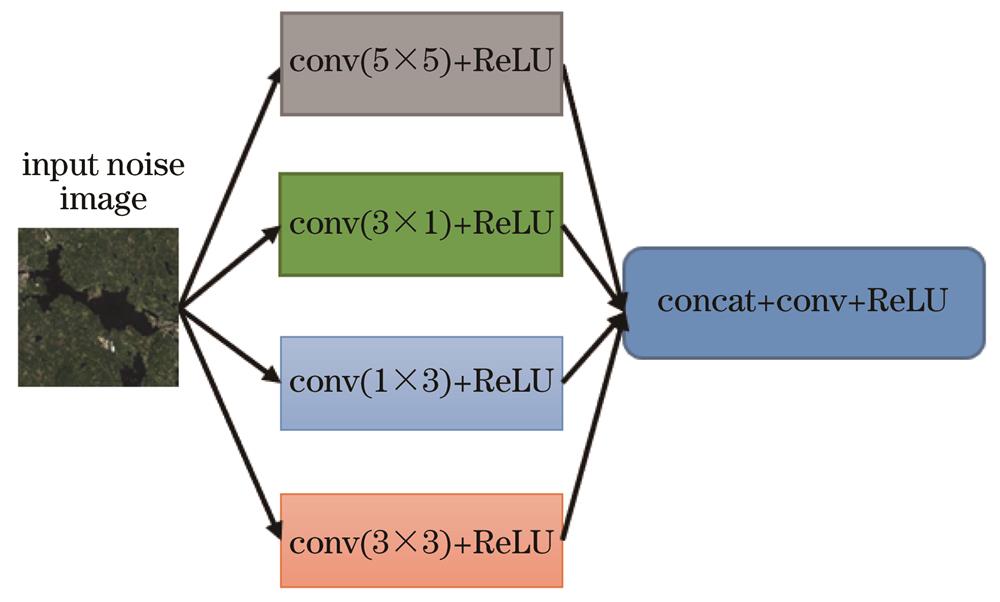
Fig. 1. Schematic diagram of asymmetric convolution kernel

Download full size

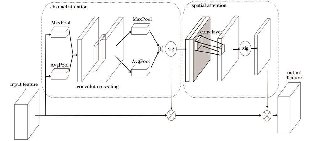
Fig. 2. Architecture of CBAM

Download full size

Fig. 3. Architecture of DCB

Download full size

Fig. 4. Architecture of MALNet

Download full size

Fig. 5. Loss curve of training model

Download full size

Fig. 6. PSNR values of different DCB layers under different modes. (a) Single background image; (b) multiple background image

Download full size

Fig. 7. Denoising effect comparison of airport image. (a) Original image; (b) noisy image; (c) denoised image obtained by WNNM; (d) denoised image obtained by SAR-BM3D; (e) denoised image obtained by SAR-CNN; (f) denoised image obtained by MALNet

Download full size

Fig. 8. Denoising effect comparison of coast image. (a) Original image; (b) noisy image; (c) denoised image obtained by WNNM; (d) denoised image obtained by SAR-BM3D; (e) denoised image obtained by SAR-CNN; (f) denoised image obtained by MALNet

Download full size

Fig. 9. Denoising effect comparison of mountain image. (a) Original image; (b) noisy image; (c) denoised image obtained by WNNM; (d) denoised image obtained by SAR-BM3D; (e) denoised image obtained by SAR-CNN; (f) denoised image obtained by MALNet

Download full size

Local	Kernel size	Stride	Padding	Channel	Pooling
$[F (0) ‑ F {(1)]}_{1}$	5×5	1	2	64
$[F (0) ‑ F {(1)]}_{2}$	3×1	1	（1，0）	64
$[F (0) ‑ F {(1)]}_{3}$	1×3	1	（0，1）	64
$[F (0) ‑ F {(1)]}_{4}$	3×3	1	1	64
F（1）	3×3	1	1	32
F（2）				32
$X_{0}$	3×3	1	1	32
$X_{1}$ ‑ $X_{2}$	3×3	1	1	32
$X_{2}$ ‑ $X_{3}$	3×3	1	1	32
$X_{3}$ ‑ $X_{4}$	3×3	1	1	32	AvgPool（2×2）
$X_{0}$ ‑ $X_{4}$	3×3	1	1	32	MaxPool（3×3）
F（3）				64
F（4）	3×3	1	1	1

Table 1. Structural parameters of MALNet

Hardware	Description
CPU	12th Gen intel（R）Core（TM）i9-12900KF @ 3.19 GHz
GPU	NVIDIA GeForce RTX 3090
Memory	32 GB
System	Windows 10
Video memory	24 GB
Language framework	Anconda + Python3.8.13 + Pytorch1.11.0

Table 2. Parameters of experimental platform

Image	$σ$	WNNM	SAR-BM3D	SAR-CNN	MALNet
Airport	20	28.87	29.28	31.85	33.42
	30	26.62	27.13	30.14	31.11
	40	26.35	26.52	29.86	29.97
	45	25.28	25.93	27.77	29.31
	50	25.17	24.01	27.67	27.82
Mountain	20	28.15	29.13	31.10	33.76
	30	26.53	27.65	30.03	31.17
	40	25.72	26.04	28.53	29.59
	45	25.14	25.99	27.17	27.85
	50	24.05	25.92	27.31	26.62
Coast	20	28.22	30.21	31.01	33.83
	30	26.63	28.52	29.43	31.58
	40	26.55	27.73	28.59	29.98
	45	25.39	26.24	26.87	28.93
	50	24.37	25.55	26.12	26.11

Table 3. Denoising level (PSNR) of each algorithm for each type of SAR image under different noise levels

Image	$σ$	WNNM	SAR-BM3D	SAR-CNN	MALNet
Airport	20	0.7929	0.8324	0.8923	0.9257
	30	0.7538	0.7826	0.8621	0.8969
	40	0.7063	0.7505	0.8669	0.8671
	45	0.6818	0.6867	0.7926	0.8309
	50	0.6821	0.6027	0.7818	0.7892
Mountain	20	0.7867	0.8354	0.9012	0.9354
	30	0.7128	0.7891	0.9010	0.9194
	40	0.6957	0.7497	0.8725	0.8963
	45	0.6708	0.7134	0.7971	0.8361
	50	0.6684	0.6808	0.8211	0.7655
Coast	20	0.7911	0.8561	0.9036	0.9253
	30	0.7187	0.7899	0.8947	0.8987
	40	0.7064	0.7587	0.8809	0.8827
	45	0.6817	0.7308	0.7437	0.8817
	50	0.6512	0.6915	0.7018	0.7939

Table 4. Denoising level (SSIM) of each algorithm for each type of SAR image under different noise levels

Image	$σ$	WNNM	SAR-BM3D	SAR-CNN	MALNet
Airport	20	6.5312	6.3112	6.8529	6.1879
	30	6.8254	6.7709	7.2964	6.3542
	40	7.1596	6.9606	7.5976	6.8793
	45	7.3177	7.2318	7.2151	6.9074
	50	7.8325	7.6321	7.4647	7.5258
Mountain	20	6.4219	6.3864	7.0158	6.0872
	30	6.8297	6.5913	7.2479	6.3173
	40	7.3541	7.1291	7.8931	6.7966
	45	7.5627	7.3945	7.9315	6.9037
	50	7.9861	7.4837	8.0147	7.5813
Coastal	20	6.5207	6.2186	6.9615	6.2157
	30	6.7896	6.4517	7.3541	6.7959
	40	7.1584	6.9526	7.7987	6.8394
	45	7.6983	7.0118	7.8424	7.0288
	50	7.9527	7.3189	7.8951	7.8198

Table 5. Image entropy of each algorithm for each type of SAR image under different noise levels unit:

b i t \cdot p i x e l^{- 1}

Xiangwei Fu, Huilin Shan, Lü Zongkui, Xingtao Wang. Synthetic Aperture Radar Image Denoising Algorithm Based on Deep Learning[J]. Acta Optica Sinica, 2023, 43(6): 0610002

Download Citation

Set citation alerts for the article

Tools

Set citation alerts for the article

Save the article for my favorites

Paper Information