In optical fiber communications, receiver design is a crucial and interdisciplinary work. Conventional receivers are functioned to map the transmitted signals from a photodetector (PD) into the bit stream^[1]. Though they can decode the bit stream transmitted, the algorithms inside the conventional receiver models are distributed and dispersed. For example, both aims and realization ways of digital dispersion compensation algorithms in fiber dispersion compensation^[2] modules and Viterbi-related decoding algorithms^[3] in decoding modules are totally different. In addition, compatibility of signals between the modules should be taken into consideration due to the dispersed algorithms in each signal. This lack of commonality and universality may result in the redesign and reconfiguration of receiver modules in different optical communication systems.

Thanks to the rapid development of integrated circuit manufacturing and distributed computing hierarchical designs, artificial intelligence (AI) technology has been surging and developing at an unprecedented speed in recent years. Not only have the traditional algorithms such as decision tree^[4], support vector machine (SVM)^[5], and K-nearest neighbors (KNN)^[6], been thoroughly researched and applied in the tasks of language translation, loan evaluation^[7], etc., but also novelty models like artificial neural networks (ANNs) of different kinds have become subjects of intensive research^[8]. Up until now, various neural networks such as convolution neural networks (CNNs)^[9–11], recurrent neural networks (RNNs)^[12], and long-short term memory modules (LSTMs) have been put forward. Due to their structural differences, CNNs have great advantages in the fields of pattern recognition^[10] and image processing^[11], while RNNs and LSTMs have been widely adapted in natural language processing (NLP) and time series processing. In recent years, various neural networks or other AI models have been applied in the fields of photonics and optics^[13]. There has been an increasing focus on optical communications, ANNs and CNNs in recognition of modulation formats^[14], eye diagrams^[15], and so on. Other models may have great applications in improving the quality of optical communication systems^[16–18]. The technology of neural networks has been integrated with the technology of optoelectronics at an unprecedented speed^[19–22].

Transformers were put forward in 2017 and have been widely and deeply researched in recent years^[23]. Due to their multi-head attention mechanisms, they show great advantages in extracting different crucial information from long time series over other models like RNNs by solving the memory decay mechanisms. Therefore, we put forward the AI-based fiber receiver model, which adopts the multi-head attention mechanism and the corresponding data collection and model training strategies. This model, once appropriately trained through data, can have a relatively greater ability of extracting and compensating distortions. Therefore, it can de-overlap the signals well and map them into the bit stream, as the conventional receivers do. Thanks to the great generalization of deep neural networks, the model can have relatively great generalization on transmission distances from 0 to 100 km. Performances of this model are numerically demonstrated and compared with conventional receivers.

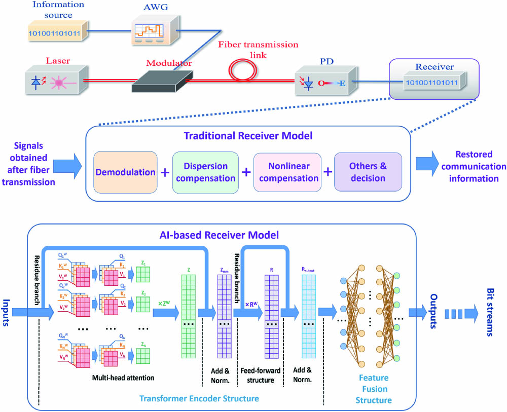
As is shown in Fig. 1, the whole communication scenario consists of information source, a laser, an intensity modulator, a fiber transmission link, and a receiver. The AI-based receiver model functions as a traditional receiver that can transfer the transmitted signals into the bit stream. Therefore, the inputs should be transmitted signals that contain fiber dispersion, nonlinear effects, and noise, while the outputs are the bit stream. Since in actual communication systems, mapping relations between bit information and communication symbols are one-by-one once fixed, communication symbols are utilized in the training process and bit information is utilized in the bit error calculation of the testing process.

In total, the AI-based receiver model consists of two different modules, including the transformer encoder structure and the feature fusion structure. Model design should originate from the conventional receiver, though most deep neural networks lack an explanation. The transformer encoder module can be viewed as the primary de-overlap module to recover the transmitted signals from intensive intersymbol interference (ISI) caused by fiber dispersion and nonlinear effects compensations that may occur during the signal propagation in the fiber. The subsequent feature fusion structure processes the data containing features extracted from the previous transformer encoder structure to better map the feature information into the predicted symbols as the model’s outputs. Further bit streams can be restored by adopting the decision rules like conventional receivers.

For the transformer encoder module, multi-head mechanisms are applied. As can be seen from Fig. 1, as the input transmitted signals come into the first module, multi-head attention mechanisms are adopted to extract the information of the overlapped and distorted signals. Since multi-head mechanisms adopt quarry, key, and value matrices to conduct convolution with signals, they will show a higher ability in extracting and storing multiple information bits over a long time duration^[23]. The residue structure is the second important structure adopted in the first transformer encoder module, which is shown as the residue branches and add and norm layers^[24]. These residue branches replicate the data and allow them to pass directly through several layers to merge with the processed ones in the subsequent layer before activation in order to prevent the potential gradient vanishing problem in training procedures.

For the feature fusion module, several layers of neurons and activation functions work together to further process the features from primarily the de-overlapped signals that were previously extracted by the transformer encoder structure to better restore the transmitted information. Taking into account both computing resources and task requirements, there are four layers, including two hidden layers with each containing 512, 1024, 1024, and 32 neurons in this module. Nonlinear activation functions, as one of the hyperparameters in this structure, are chosen to be rectified linear unit (ReLU) in order to avoid the slow weights update during the later parts of the learning procedures.

After that, the decision rules, which are closely related to the bit-symbol mapping in the transmitter parts of optical communication systems, can be adopted to further turn the predicted symbols as the outputs of the AI-based receiver model into the bit streams.

Since the AI-based receiver model learns from large amounts of data, establishment and configurations of the data set are of great significance as well. The whole data set consists of training data, validation data, and testing data. In each data sample, a total of four attributes are included, which refer to modulation format (MF), symbol rate (Rs), transmission distance (D), and signal-to-noise ratio (SNR). These four attributes are called a quadruple and can be denoted as (MF, Rs, D, and SNR). Once the value of the quadruple is determined, the data collection systems, whose important properties are listed in Table 1, are completely chosen. In this paper, MF ranges from on–off keying (OOK) to 4-pulse amplitude modulation (PAM4). Rs ranges from 10 GBaud and 20 GBaud to 40 GBaud. D ranges from 1 to 100 km, with an interval of 1 km in both the training and validation data sets, while D ranges from 0.5 to 99.5 km, with an interval of 1 km in the testing data set. SNR ranges from 0 to 16 dB and +inf in OOK, while SNR ranges from 0 to 20 dB and +inf in PAM4. The sampling rate is 8 times higher than that of the symbol rate. The model will then be trained separately for different MF, Rs, and SNR by using data originated from signals transmitted from different distances, so that the model is able to obtain relatively good generalization ability over transmission differences.

All data utilized for the model’s training and testing follow the format described in Fig. 2. In general, the input data are made up of the sampling points from the transmitted signals, while the targets are made up of the correct symbol values. The notation ‘s’ in this figure represents all the sampling points from the waveforms corresponding to each symbol, while it represents the symbol value in the targets. For each data sample, it contains both input and target. The inputs contain three dimensions, which are shown on the left side in Fig. 2. The first dimension is the index of symbols, each containing 16 values, with the former 8 values representing the real parts of the 8 sampled points for each symbol and the latter 8 values representing the imaginary parts, meaning k equals 8 in Fig. 2. The second index is the index of sampling points in one data sample. Here, there are altogether 4096 sampling points from 32 symbols that form one data sample, meaning n equals 32 in Fig. 2. The third dimension is the data sample index in one batch for the model’s training and testing. In total, 128 data samples exist in one batch, meaning m equals 128. In contrast, the data of the targets have two dimensions, a symbol index and a group index, whose meaning is the same as inputs. As for the scale of the data in the whole data set, it varies with respect to the training data set, the validation data set, and the testing data set.

As for the training of this model, the loss function is chosen to be normalized mean square error (NMSE), and the optimization method is determined to be adaptive momentum stochastic gradient descend method (ADAM)^[25], with the batch size equaling 128. Figure 3 shows one example of the training procedure of the model with respect to quadruple (MF=PAM4, D=60km, Rs=10GBaud, SNR=+inf). Judging from the convergence curve, the NMSE loss decreases as the epoch increases. The slope of the curve changes from steep to horizontal, which indicates the converging results. Fluctuations may exist in the curve, and this implies the unflatness of the surface of the loss. In addition, from Figs. 3(b)–3(k), the outputs distribution progressively reaches the targeted symbol values as the epoch goes.

In order to test the performances of the AI-based receiver model, BER-SNR diagrams are utilized, which have been widely used in applications in conventional communication receivers. SNR evaluates the relative signal power with respect to noise power, while BER evaluates the number of the wrongly detected.

Baseline or reference results are obtained from conventional receivers with hard detection. In contrast, these conventional receivers contain both chronic dispersion compensation and nonlinearity equalization algorithms or devices. Without losing generality, the traditional receivers compensate for fiber dispersion of the 50.5 km transmission before bit detection. In the real transmission circumstances, this compensation method can either be dispersion compensation fiber (DCF), with the total dispersion value equaling 845.875 ps/nm in the optical domain, or the corresponding finite inpulse response (FIR) filter in the electronic domain. According to the theory of telecommunications, noise suppression algorithms or devices are usually adopted in conventional receivers before bit detection^[1]. These can effectively improve the detection accuracy. Please note that the SNR values used in Fig. 4 refer to the SNR before the noise suppression algorithms filters in order to conduct fair comparisons, since the AI-based receiver model conducts detection by utilizing the signals without the processes of noise suppression algorithms. Here, two conventional receiver models, one with noise suppression algorithms and the other without noise suppression algorithms, are both adopted as the baseline models in comparison with the AI-based receiver model.

All results shown as the formats of SNR-BER diagrams are depicted in Fig. 4. For the quadruple described above, MF and Rs are plotted separately in each subfigure, while SNR and D are depicted as two axes to form the horizontal plane of each subfigure, respectively. The color turns yellow or red when BER increases, while turning blue or purple as BER decreases. For the relatively small BER (which is less than 10−6), a dark purple color is utilized to cover this region.

The analysis of these BER-SNR diagrams can center on how the quadruple attributes affect the performance of the model. By comparing the diagrams in Figs. 4(a3)–4(c3) with Figs. 4(d3)–4(f3), the AI-based model performs better in OOK signals than in PAM4 signals with the same configuration of the other three attributes in the quadruple. First, the waveform complexity of the PAM4 is higher than that of the OOK. Second, though with the same dispersion and nonlinearity for the same distance, PAM4 signals experience more intense distortions. Third, for PAM4 signals, the Hamming decision distance between each set of two neighboring symbols is less than that of the OOK. By comparing Fig. 4(a3) with Figs. 4(b3) and 4(c3) or Fig. 4(d3) with Figs. 4(e3) and 4(f3), one can clearly see how the symbol rate affects the performance of the AI-based fiber model. With the increase of symbol rate, the difficulty of mapping transmitted signals into the targeted bit stream also increases.

In contrast with the modulation format and symbol rate, which have relatively uniform or monotonal effects on the performances of the model, the last two attributes, SNR and distance, may cause rather complicated effects. As for the SNR, the overall rule is that the higher the SNR, the better the model predicts. Unlike fiber dispersion or other nonlinear effects during fiber propagation, which can be compensated for, noise is irreversible and cannot be completely removed. It will cause the turbulence on signals, which may trigger the AI-based model to misclassify as long as the turbulence is large enough and can even cause a dramatic decrease in the performance of the model. From Fig. 4(b3), at a distance equaling around 80 km, the BER ranges from 10−2 to 10−6 and from 0 to 20 dB. As for the transmission distances, its effect should be the same for the specific SNR, which means that the contour lines in Fig. 4 should be horizontal under ideal circumstances, in which the distance generalization ability equals infinity. However, even with relatively good distance generalization, the unflatness also exists and cannot be ignored, especially for a higher symbol rate and higher-order modulation formats. As can be seen from Figs. 4(a3) and 4(d3), the BER contour line is almost horizontal during the transmission distances when the SNR is higher and the symbol rate is relatively lower. This indicates that the AI-based receiver model shows relatively better distance generalization for those signals that contain less noise and are transmitted at a relatively lower symbol rate. However, with the increasing of either noise power or symbol rate, the contour lines tend to lose their horizontal shapes and gradually become irregular curves, which indicates the relatively poorer distance generalization for the model under these circumstances. This is because either a high level of noise or symbol rates may increase both uncertainty and distortion differences over the signals transmitted at different distances. Hence, it will be more difficult for the model to maintain the same distance generalization ability in cases where both noise power and symbol rate are lower.

The prediction accuracy and distance generalization ability of the AI-based receiver model can be illustrated more vividly and precisely as compared with the traditional receiver model by comparing the subfigures in the third column with the first and second columns. As for the prediction accuracy, the overall performance of the AI-based receiver model is better, especially for lower BER cases. From Fig. 4(a3), the BER of the AI-based model is around 10−3 for most transmission distances, while the BER of the conventional model with noise suppression algorithms is 10−1 when SNR equals 0 dB, the conventional model without noise suppression algorithms. However, this BER gain decreases when the bit rate becomes higher, and the modulation format turns out to be more sophisticated, since the fitting difficulties become higher for the AI-based receiver model. Distance generalization can also be clearly seen by comparing the shapes of the contour line. In detail, the contour lines show more flatness with respect to transmission distances in the AI-based receiver model than in the other two conventional models. For conventional receivers, since compensation work is done for 50.5 km, its relatively distance-sensitive property makes the system compensate more or less for other transmission distances, which will cause the incomplete de-overlapping of the signals. Therefore, the contour lines bend toward 50.5 km. In contrast, due to the relatively better distance generalization ability, the counter lines show more flatness with respect to the transmission distances in the AI-based receiver model. For higher symbol rates and more sophisticated modulation formats, since more intense distortions need to be compensated for, the counter lines bend to a relatively greater extent in all the three models.

The time complexity of this model is related to the scale of its learnable parameters, such as quarry, key, and value matrix representations and the scale of weight matrices of the subsequent layers. On average, models with a larger scale of learnable parameters can obtain stronger regression abilities. Under this circumstance, one effective way of either improving the prediction precision of the model or extending the model’s applications on more sophisticated communication systems is to enlarge its learnable parameters.

In conclusion, an AI-based receiver model containing a multi-head attention mechanism was put forward in this paper. Through appropriate training, it can progressively learn to map the transmitted signals into the bit stream under different transmission circumstances. Three main advantages can be obtained. First, there is no need to design different compensation modules for fiber dispersion thanks to the model’s distance generalization ability, which greatly improves the compatibility of the receivers. Second, with the increase of the power of noise, the prediction performance of the AI-based model does not fall down much compared with conventional receivers. Third, this model can be further applied as the basis for other transmission quality evaluation models in short-distance fiber optical communications. Future attention will be focused on further improving the performance of the model and extending its application into higher-order modulated signals.

References

[1] G. Keiser. Optical Fiber Communications(2000).
[2] S. Ramachandran. Fiber Based Dispersion Compensation(2007).
[3] G. D. Forney. The Viterbi algorithm. Proc. IEEE, 61, 268(1973).
[4] J. R. Quinlan. Induction of decision trees. Mach. Learn., 1, 81(1986).
[5] C. Cortes, V. Vapnik. Support-vector networks. Mach. Learn., 20, 273(1995).
[6] T. Cover, P. Hart. Nearest neighbor pattern classification. IEEE Trans. Inf. Theory, 13, 21(1976).
[7] C. M. Bishop. Pattern Recognition and Machine Learning(2006).
[8] A. K. Jain, J. Mao, K. M. Mohiuddin. Artificial neural networks: a tutorial. Computer, 29, 31(1996).
[9] S. Albawi, T. A. Mohammed, S. Al-Zawi. Understanding of a convolutional neural network. International Conference on Engineering and Technology (ICET), 1(2017).
[10] S. Lawrence, C. L. Giles, A. C. Tsoi, A. D. Back. Face recognition: a convolutional neural-network approach. IEEE Trans. Neural Netw., 8, 98(1997).
[11] L. Xu, J. S. Ren, C. Liu, J. Jia. Deep convolutional neural network for image deconvolution. Adv. Neural Inf. Process Syst., 27, 1790(2014).
[12] T. Mikolov, M. Karafiát, L. Burget, J. Černocký, S. Khudanpur. Recurrent neural network based language model. Eleventh Annual Conference of the International Speech Communication Association(2010).
[13] Y. Shen, N. C. Harris, S. Skirlo, M. Prabhu, T. Baehr-Jones, M. Hochberg, X. Sun, S. Zhao, H. Larochelle, D. Englund, M. Soljačić. Deep learning with coherent nanophotonic circuits. Nat. Photonics, 11, 441(2017).
[14] E. E. Azzouz, A. K. Nandi. Modulation Recognition Using Artificial Neural Networks, 132(1996).
[15] J. A. Jargon, X. Wu, A. E. Willner. Optical performance monitoring using artificial neural networks trained with eye-diagram parameters. IEEE Photon. Technol. Lett., 21, 54(2008).
[16] B. Karanov, M. Chagnon, F. Thouin, T. A. Eriksson, H. Bülow, D. Lavery, L. Schmalen. End-to-end deep learning of optical fiber communications. J. Light. Technol., 36, 4843(2018).
[17] D. Wang, Y. Song, J. Li, J. Qin, T. Yang, M. Zhang, X. Chen, A. C. Boucouvalas. Data-driven optical fiber channel modeling: a deep learning approach. J. Light. Technol., 38, 4730(2020).
[18] F. N. Khan, Q. Fan, C. Lu, A. P. T. Lau. An optical communication’s perspective on machine learning and its applications. J. Light. Technol., 37, 493(2019).
[19] X. Jin, S. Li, Z. Xu. Compensation of turbulence-induced wavefront aberration with convolutional neural networks for FSO systems. Chin. Opt. Lett., 19, 110601(2021).
[20] S. Xu, W. Zou. Optical tensor core architecture for neural network training based on dual-layer waveguide topology and homodyne detection. Chin. Opt. Lett., 19, 082501(2021).
[21] L. Yang, L. Zhang. Recent progress in photonic reservoir neural network. Chin. J. Lasers, 48, 1906001(2021).
[22] L. Zhao, Z. Han, F. Zhang. Research on stereo location in visible light room based on neural network. Chin. J. Lasers, 48, 0706004(2021).
[23] A. Vaswani, N. Shazeer, N. Parmar, J. Uszkoreit, L. Jones, A. N. Gomez, Ł. Kaiser, I. Polosukhin. Attention is all you need. 31st Conference on Neural Information Processing Systems(2017).
[24] S. Targ, D. Almeida, K. Lyman. Resnet in resnet: generalizing residual architectures(2016).
[25] D. P. Kingma, J. Ba. Adam: a method for stochastic optimization(2014).
Set citation alerts for the article
Please enter your email address
© Copyright 2018-2021 | Chinese Laser Press. All Rights Reserved 沪ICP备15018463号-20