Cholesteric liquid crystals (CLCs) are one-dimensional, self-assembled photonic band-gap materials. Their helical structure, easily deformable by external fields, produces a modulation of the refractive indices along the helical axis. This induces Bragg reflection in a range of wavelengths close to the helical pitch, for circularly polarized light of the same handedness as the CLC structure ^[1]. In addition to its unique optical properties, CLC is one of the two photonic band gap structures for which exact analytic solutions of the Maxwell’s equations exist for light propagating along the helical axis ^[2]. The analytic solution for CLCs was first derived by Mauguin in 1911 ^[3], for the case when the pitch is much larger than the incident light wavelength, and was later formulated more generally by Oseen in 1933 ^[4] and de Vries in 1951 ^[5]. Several authors have since proposed analytic solutions for infinite or semi-finite bulk CLCs ^[6,7], solving Maxwell’s equations in more general anisotropic stratified systems, such as smetic liquid crystals ^[8], or for oblique incidence ^[9].

Selective reflection and its easily deformable structure makes CLC slabs suitable for a variety of applications, such as tunable filters, mirrors, polarizers, smart windows ^[10], etc. Depending on the application, the thickness of a CLC slab would typically vary from a few to hundreds of micrometers. Thicker slabs are required for devices operating at longer wavelengths, such as infrared reflectors. The reflection and transmission spectra of a finite CLC slab have not been derived analytically. Typically, numerical methods, such as the Berreman 4×4 method ^[11,12] or the Jones matrix method ^[13], are used for such calculations. However, these propagation matrix methods are not suitable for thick samples since they tend to become unstable ^[13,14]. Numerical instabilities appear in the reflection band due to terms increasing exponentially with the cell thickness. For instance, double-precision computation results in diverging errors inside the band-gap for samples thicker than 100 pitches of the cholesteric ^[13].

Following preliminary work ^[15], we present here analytic expressions for the radiation fields of the transmitted and reflected light for normal incidence on a CLC slab of finite thickness. These allow us to overcome the problems of numerical errors. Indeed, the reflected and transmitted waves can be calculated for a sample of arbitrary thickness, enabling accuracy far beyond the limitation of numerical propagation matrix methods.

The wave equation describing the electric field inside a CLC is obtained from Maxwell’s equations. It is solved in a rotating frame that follows the CLC’s helical structure. The solution is then transformed into the lab coordinate system.

For the sake of completeness we derive the solution from the first principles rather than citing existing results.

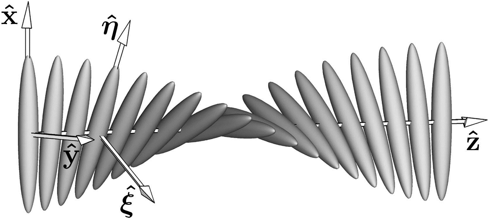
Typically, CLCs consist of molecules whose average orientation depends on position. The molecules are assumed to be effectively cylindrically symmetric; the orientation of a molecule is taken to be the orientation of the axis of symmetry. The average direction of the symmetry axes of the molecules, the nematic director, is described by a unit vector n^, which is perpendicular to the helical axis of the CLC. The helical structure of the CLC is shown in Fig. 1.

The lab coordinate system (x^,y^,z^) is chosen so that the helical axis points along the z^ direction. In this frame the director’s coordinates are (cos(qz),sin(qz),0), where q is the helical wave number, related to the helical pitch p by q=2π/p.

In this work we assume that the director traces out a right-handed helix. Similar procedure can be used for a left-handed CLC. The rotating coordinate system (η^,ξ^,z^) follows the rotation of the director n^. The rotating frame is related to the lab frame via the transformation

In the rotating frame the director is constant, pointing along η^=(1,0,0). In this frame, the dielectric tensor is diagonal, given by ε¯¯r=ε⊥I¯¯+(ε∥−ε⊥)η^η^, where ε∥ and ε⊥ are the principal values of the dielectric constant parallel and perpendicular, respectively, to the director.

We assume a plane wave solution with the electric field in the x^−y^(ξ^−η^) plane: E=E(z)ei(kz−ωt). The wave equation is then reduced to where the prime indicates derivative with respect to the z-coordinate.

Assuming that the light in the rotating frame is elliptically polarized with constant amplitude, i.e., E(z)=E∥η^+E⊥ξ^, and noting that η^′=qξ^ and ξ^′=−qη^, one obtains where α=λ0/p is the dimensionless wavelength and n is the refractive index. Solving for the eigenmodes gives

This indicates that there exist two propagating normal modes, with two waves propagating in the positive and two in the negative z-direction: where ε¯=(1/2)(ε∥+ε⊥) and δ=(1/2)(ε∥−ε⊥).

Positive (negative) roots of expressions (5) and (6) correspond to propagation in the positive (negative) direction along the z^ axis. Having determined the refractive indices, one can write the solution for the electric fields inside the CLC. In the rotating frame we denote η^=[10], ξ^=[01], then The “+” and “−” superscripts indicate propagation in the z^ and −z^ directions, respectively. A and B are directly related to the ellipticities of the normal modes and are given by or, which is the same, as

The corresponding wave vectors are given by k1,2=2πn1,2/λ0. Here n1=n1+ and n2=n2+.

Equation (6) shows that n22 is negative when pε⊥<λ0<pε∥, which implies that n2 is imaginary and E2 is a nonpropagating mode. This wavelength range corresponds to the bandgap, the selective reflection band of the CLC, for circularly polarized light of the same handedness as the CLC structure.

In the lab frame, we denote x^=[10], y^=[01], and the normal modes are as follows: where E1+, E1−, E2+, and E2− are constants. In the lab frame, each normal mode is thus a linear combination of left and right circularly polarized light, with different amplitudes and wavenumbers.

Having identified the normal modes, we next solve the boundary problem for a CLC cell of finite thickness d. The CLC is confined between parallel plane substrates with refractive indices nsi on the side of the incident light and nst on the other. We assume that our substrates are semi-infinite; this is to avoid additional Fresnel reflections from air-substrate interfaces. Fresnel reflections are discussed in ^[16]. The helix axis is perpendicular to the substrate surfaces. The lab coordinate is chosen so that the director is along the x^ direction, and z=0 at the CLC surface where light is incident (see Fig. 2).

The complex electric fields in the lab frame, corresponding to the incident Ei, reflected Er, and transmitted Et light waves, can be written as follows: The magnetic fields can be expressed in terms of the electric fields as H=−i∇×E/(ωμ0).

The boundary conditions are the continuity of the tangential components of the electric and magnetic fields. The first set of equations relating Ei, Er and the fields inside the CLC is obtained from satisfying the boundary conditions at the interface z=0. Similarly, the second set of equations relating Et and the fields inside the CLC is obtained at the interface z=d. Eliminating the fields inside the slab gives the relations between the components of the incident, reflected, and transmitted waves: The transfer matrices P¯¯ and Q¯¯ are 2×2 matrices. Their elements are given in the Appendix A. 0¯¯ denotes a zero 2×2 matrix.

The transmitted and reflected fields can be obtained explicitly from the incident field to give Analytic expressions for the elements of P¯¯−1 and Q¯¯P¯¯−1 matrices together with the detP¯¯, needed to invert P¯¯, are also given in the Appendix A. These analytic expressions relating the incident, reflected and transmitted fields are one of our key results.

Figure 3 shows the transmitted and reflected intensities from light incident on a CLC slab of thickness d=100p. If the intensities of reflected and transmitted light are calculated numerically, say by evaluating P¯¯−1 and Q¯¯P¯¯−1, numerical errors arise, which make the solution in the bandgap unreliable, as indicated in Fig. 3(a). We discuss the origin of these errors below. If we use our analytic results for P¯¯−1 and Q¯¯P¯¯−1, no such errors arise, enabling the accurate determination of the response of even very thick cells accurately, as shown in Figs. 3(b) and 4.

Figure 4 shows the spectra of a CLC cell with d=10,000p, and in Figs. 5 and 6, the reflection spectrum of the same cell is shown in details at the center of the reflection band and near its edge. The parameters used are nsi=nst=ns=1.6, ε⊥=2.25, ε∥=2.89, p=380nm. We have chosen the principal values of the dielectric tensor so that they would correspond to typical refractive index values in nematics. In our paper, the refractive indices corresponding to the dielectric constant values 1.5 and 1.7 (in 5CB, the values are approximately 1.53 and 1.72 at room temperature). We have chosen the substrate index to be the average of these, 1.6, in order to minimize cavity effects. The incident electric field was chosen to be linearly polarized in the x^ direction for these calculations. Equivalent calculations can be carried out for other polarizations.

We now turn to the origin of numerical errors and how they are avoided by use of our analytic results. Each element of the transfer matrices P¯¯ and Q¯¯ (see Appendix A) contains terms of the form e−ik2d that diverge when n2 is imaginary, −ik2d is positive, and d is sufficiently large. These become the dominant terms and determine the order of magnitude of the elements of the two propagation matrices. Since every element contains e−ik2d, the detP¯¯ might be expected to contain e−i2k2d as a dominant term. Yet analytic calculations show that terms e−i2k2d in detP¯¯ always cancel out, making e−ik2d the dominant term. This is a consequence of the specific structure of the propagation matrices. One can thus see that P¯¯ and detP¯¯ are of the same order of magnitude and P¯¯−1 is typically of the order of unity. Errors result from the direct numerical calculation of detP¯¯, where products are formed of e−i2k2d and a number that is not exactly zero, but is within machine precision of zero. For a thick cell, e−i2k2d can be orders of magnitude larger than the machine epsilon, adding significant errors to the final value of the determinant. Similar behavior occurs during the calculation of Q¯¯P¯¯−1: the dominant term e−ik2d is canceled out if the product is taken analytically, but does not cancel exactly numerically. For nonabsorbing CLCs, the reflected light intensity is simply the difference of the incident and transmitted intensities; thus calculating only P¯¯−1 is sufficient. To calculate reflection from an absorbing cell, one necessarily needs to use both P¯¯−1 and Q¯¯P¯¯−1.

Numerical propagation methods, such as the classical Berreman 4×4 method ^[11], show errors of a similar origin, making numerical modeling of thick CLC samples problematic ^[17]. We note that for thinner cells, such as d=25p, the Berreman 4×4 method and analytic solution give an identical spectrum.

Analytic solutions of the wave equation in the bulk, together with boundary conditions, allow analytic expressions for the transmitted and reflected fields for CLC cells in terms of the incident field. Although equations are long and cumbersome, our approach allows the calculation of the reflection and transmission spectra for arbitrarily thick CLC cells in the case of normally incident light. This scheme overcomes the limitations of existing numerical propagation methods.

References

[1] P. Collings, M. Hird. Introduction to Liquid Crystals: Chemistry and Physics, the Liquid Crystals Book Series(1997).
[2] V. Beliakov. Diffraction Optics of Complex-Structured Periodic Media, Partially Ordered Systems(1992).
[3] C. Mauguin. Sur la représentation géométrique de Poincaré relative aux propriétés optiques des piles de lames. Bull. Soc. Fr. Mineral. Cristallogr., 34, 6-15(1911).
Sabrina Relaix, Mykhailo Pevnyi, Wenyi Cao, and Peter Palffy-Muhoray, "Analytic solutions of the normal modes and light transmission of a cholesteric liquid crystal cell," Photonics Res. 1, 58 (2013)