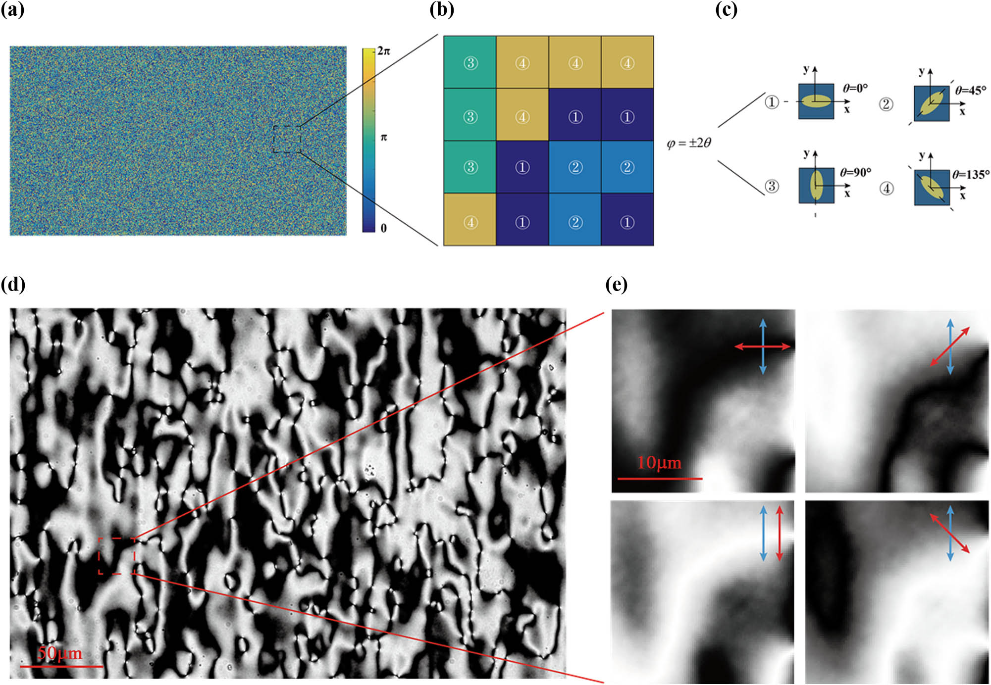
Fig. 1. Design of LC metasurface diffuser. (a) Designed phase distribution of the LC metasurface diffuser. (b) Local phase distribution of the LC metasurface diffuser with the four-order phase. (c) The four LCMs with different rotation angles corresponding to the four-order phase distribution. (d) The POM image of the metasurface diffuser. (e) The local magnification POM images under different polarization states, and the blue and red arrows denote the input and output polarization states of light.

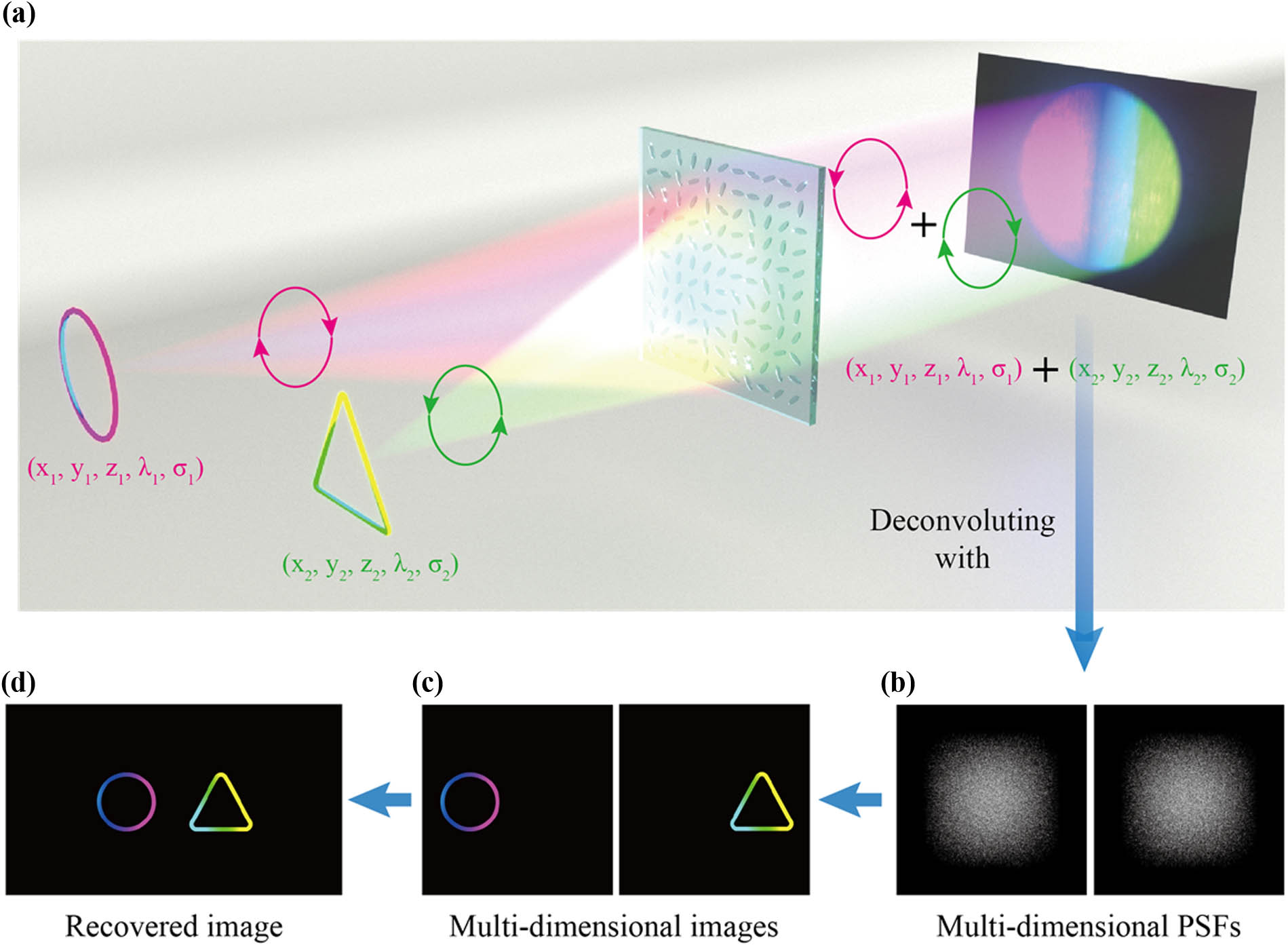
Fig. 2. Schematic of the spatial–spectral–polarization meta-optical imaging system. (a) Light from two multispectral objects with different spatial and polarization (left, left-circularly polarized; right, right-circularly polarized) information propagating through the designed LC metasurface diffuser generates a speckle pattern on a monochromatic camera. (b) Speckle patterns produced by two-point objects with respective spatial and polarization information of the two multi-dimensional objects, taken as corresponding multi-dimensional PSFs. (c) Reconstructed multi-dimensional images from the monochromatic speckle images using corresponding PSFs. (d) The recovered image of the two objects by superimposing individual reconstructed images.

Fig. 3. Spatial resolution of the MCI system. (a) Schematic diagram of the experimental setup. (b) The diagonal length of the DMD chip used in the projector is 0.55 in., and the pixel size is 14 μm. (c) The resolution chart loaded on the projector and the recovered images. The gaps of each line are 1, 2, and 3 pixels, respectively. (d) Intensity profile of lines in (c). Scale bar: 50 μm in (c).

Fig. 4. Schematic of MCI’s multispectral imaging. (a) The raw speckle patterns generated by different chromatic objects. (b) The PSFs generated by a central point object with corresponding colors. (c) The images reconstructed from the speckle patterns using corresponding PSFs. (d) The ground truth pictures projected on the projector, which are projected respectively. (e) The full reconstructed image by superimposing seven individual spectral images in (c). Scale bar: 1000 μm in speckle patterns and PSFs, and 100 μm in reconstructed images.

Fig. 5. Schematic of MCI’s polarization selective characterization. (a) Schematic diagram of the experimental setup. The first pair of the polarizer and quarter-wave plate converts incident light to LCP light (indicated by the red rotation spinning arrow). Then the LCP light transmits through the metasurface and is converted to RCP light (indicated by the blue rotation spinning arrow). Limited by the polarization conversion efficiency of the metasurface, some LCP light is left in transmitted light. The second pair of the polarizer and the quarter-wave plate is employed to remove LCP light. (b) has the same experimental setup as (a), except the rotation angle of two quarter-wave plates is changed for the generation and removal of RCP light. (c) The raw speckle patterns with different polarization (blue for RCP, red for LCP). (d) The PSFs with different polarization. (e) The reconstructed images from the speckle patterns by deconvolution with PSFs of the same polarization. (f) The reconstructed images from the speckle patterns by deconvolution with PSFs of the orthogonal polarization (there are two rotation spinning arrows in the upper left; the left and right arrows indicate polarization of speckle pattern and PSF). Scale bar: 1000 μm in speckle patterns and PSFs, and 100 μm in reconstructed images.

Fig. 6. Schematic of MCI’s 5D imaging. (a) Schematic diagram of the experimental setup. Two objects (left and right) are projected simultaneously and transmitted through a diaphragm and polarizer, which blocks stray light and converts to linear polarization. M1, M2, and M3 are mirrors, and M1 and M2 reflect the left object to another path. Quarter-wave plates circularly polarize both objects. The two quarter-wave plates are set to orthogonal rotation angles to produce different circularly polarized objects. Following M3 reflects the left object to the main path and the beam splitter superimposes both objects together. Then the superimposed beam transmits through the metasurface and is recorded by the camera. (b) The superimposed speckle pattern of two objects with different 5D information. (c) The individual measured PSF of the right path and the reconstructed image from the superimposed speckle pattern by deconvolution. (d) The individual measured PSF of the left path and the reconstructed image from the superimposed speckle pattern by deconvolution. Scale bar: 1000 μm in speckle patterns and PSFs, and 100 μm in reconstructed images.

Fig. 7. Wavelength resolution comparison of random and focus phase profiles. We simulate the imaging results under these two phase profiles with a center wavelength of 532 nm and deconvolve these images with their PSFs of varying wavelengths. (a) and (c) are the reconstructed results under different PSFs with corresponding phase profiles at different wavelengths. (b) and (d) show the simulated PSFs for each phase profile. (e) The Jaccard index of the reconstructed results compared with the ground truth image. (f) The Pearson correlation coefficient of the reconstructed results compared with the ground truth image.

Fig. 8. Spatial resolution comparison of random and focus phase profiles. We simulate the imaging results under these two phase profiles at the distance of 15 cm along the z axis and deconvolve these images with their PSFs varying the distance along the z axis. (a) and (c) are the reconstructed results under different PSFs at different depths with corresponding phase profiles. (b) and (d) show the simulated PSFs for each phase profile. (e) The Jaccard index of the reconstructed results compared with the ground truth image. (f) The Pearson correlation coefficient of the reconstructed results compared with the ground truth image.

Fig. 9. For LCP incidence, the Pearson correlation coefficients between PSFs with different object depths and wavelengths of incidence.

Fig. 10. For RCP incidence, the Pearson correlation coefficients between PSFs with different object depths and wavelengths of incidence.

Fig. 11. Axial resolution experimental result. (a) Scheme of z-direction resolution measurement. Two objects with different distances from the diffuser are imaged respectively, and two images are added together as the pattern to recover. (b) Different PSFs measured from different distances and corresponding reconstructed images. (c) The Pearson correlation coefficient of the reconstructed results compared with the image of the original location. Scale bar: 1000 μm in PSFs and 100 μm in reconstructed images.

Fig. 12. Test of memory effect range. (a) Scheme of memory effect range measurement. Objects are shifting out of the original position along with the projector moving, and the moving step is 0.5 mm. (b) Reconstructed images of objects in different positions. (c)–(h) Enlarged images of (b). Scale bar: 100 μm.