Snapshot multi-dimensional computational imaging through a liquid crystal diffuser

Yunsong Lei; Qi Zhang; Yinghui Guo; Mingbo Pu; Fang Zou; Xiong Li; Xiaoliang Ma; Xiangang Luo

doi:10.1364/PRJ.476317

Abstract

Multi-dimensional optical imaging systems that simultaneously gather intensity, depth, polarimetric, and spectral information have numerous applications in medical sciences, robotics, and surveillance. Nevertheless, most current approaches require mechanical moving parts or multiple modulation processes and thus suffer from long acquisition time, high system complexity, or low sampling resolution. Here, a methodology to build snapshot multi-dimensional lensless imaging is proposed by combining planar-optics and computational technology, benefiting from sufficient flexibilities in optical engineering and robust information reconstructions. Specifically, a liquid crystal diffuser based on geometric phase modulation is designed to simultaneously encode the spatial, spectral, and polarization information of an object into a snapshot detected speckle pattern. At the same time, a post-processing algorithm acts as a special decoder to recover the hidden information in the speckle with the independent and unique point spread function related to the position, wavelength, and chirality. With the merits of snapshot acquisition, multi-dimensional perception ability, simple optical configuration, and compact device size, our approach can find broad potential applications in object recognition and classification.

1. INTRODUCTION

Multi-dimensional optical imaging systems exploit different degrees of freedom of scattering photons from an object scene, such as polarization, depth, and spectrum, to reveal different information [1 –3]. For instance, spectral characteristics reflect the elemental composition, while the polarimetric characteristics contain the surface’s roughness and conductance [4]. The information can be helpful for object inspection and classification in remote sensing and industry applications. However, most existing approaches require mechanical moving parts or multiple modulation processes (e.g., polarizers of different orientations, diffractive gratings, or spectrum filters), which leads to long acquisition time, large volume size, high system complexity, or low sampling resolution.

In recent years, lensless imaging systems have gradually unfolded their advantages compared with traditional lens-based imaging systems. Unlike the point-to-point imaging manner in the latter systems, lensless imaging systems, acting as new paradigms in imaging, are replacing the conventional lenses with encoding masks and directly recording the coded pattern of an object on the sensor. Then after the post-process reconstruction, the information of the object can be recovered. Benefiting from this typical architecture, lensless imaging systems are usually more flexible, light weight, and with less cost than traditional lens-based imaging systems. It has been demonstrated that lensless imaging systems can be used in super-resolution imaging [5,6], three-dimensional imaging [7,8], multispectral [9] and hyperspectral imaging [10], and so on. Diffuser-based scattering imaging has drawn attention since much optical field information can be retrieved during the scattering process. However, there will be a random speckle in the transmittance of conventional diffusers [11], and their optical properties may be unstable with time [12], which makes the scattering effect of the conventional diffuser unpredictable and unrepeatable. Therefore, the time-consuming and tedious characterizations are unavoidable before utilization. Furthermore, due to the limited optical field engineering ability, it is also a great challenge to realize multiple-dimensional imaging for conventional lensless imaging systems owing to the wavelength and polarization insensitivity.

Digital optics could play an important role to conquer these challenges. Digital optics is a new concept that leverages discrete micro-/nano-optical elements to realize optical field manipulation with higher flexibility and resolution. As a core of digital optics, metasurfaces are planar devices comprising arrays of subwavelength meta-atoms. By locally tailoring the geometries of each meta-atom, the metasurface can manipulate the phase, amplitude, and polarization at will [13 –24]. The metasurface-based devices have been successfully demonstrated and utilized in numerous applications, e.g., light-field imaging [16], depth sensing [25], planar synthetic aperture [26], polarization detection and imaging [27,28], multispectral imaging [29], and wide field-of-view imaging and detection [18,30]. The concept of the metasurface diffuser has been well established lately to achieve high-resolution bio-imaging [31] and complex optical field imaging [32]. Compared with the conventional diffuser, the predesigned metasurface diffuser significantly simplifies the characterization procedure and shows stable and reliable optical properties. More importantly, by exploiting sensitivities of wavelength and polarization at subwavelength scales, the metasurface has the potential to realize multi-dimensional imaging [33]. Nevertheless, preparing the metasurfaces comprising great nano-pillars or nano-holes is facing enormous challenges, especially in large-area manufacturing. Alternatively, a common and straightforward approach is to develop the geometric phase elements with controllable liquid crystal (LC) orientations [34 –38]. On the one hand, the gradual maturity of LC production lines provides low-cost and large-scale production. On the other hand, compared to conventional diffraction optical elements, LCs also revealed unparalleled superiority in terms of operation efficiency, processing difficulty [39], and wavelength-polarization sensitivity.

Sign up for Photonics Research TOC. Get the latest issue of Photonics Research delivered right to you！Sign up now

In this paper, we propose and demonstrate the concept of multi-dimensional computational imaging (MCI) by combining the principles of both lensless computational imaging and metasurface optics. A flat LC-based diffuser fabricated through a standard photoalignment technology and a digital micro-mirror device (DMD) is used to encode spatial–spectral–polarization five-dimensional (5D) object information. The generated point spread functions (PSFs) exhibit linear translation invariance within the memory effect range, which promises the post-processing algorithm to recover two-dimensional information on the $x - y$ plane. The variation of depth along the $z$ axis will result in phase delays, leading to different PSFs with low correlation, which makes depth information able to be retrieved. Owing to the spin-reversed wavefront coding and dispersive diffraction character of the LC-based geometric phase diffuser, PSFs among different chirality and wavelength are highly irrelevant, benefiting to reveal polarization and spectrum information. Therefore, MCI can be easily achieved by the conventional deconvolution technique. Our proposal has been demonstrated in the visible band, with the merits of snapshot acquisition, multi-dimensional perception ability, simple optical configuration, compact device size, and high fabrication efficiency.

2. PRINCIPLE AND METHODS

A. Geometric Phase and LC Metasurface Diffuser Design

The designed metasurface diffuser is composed of anisotropic liquid crystal molecules (LCMs), based on the Pancharatnam–Berry (PB) phase [40,41], which is also called the geometric phase. The transmission property of the LCMs with a fast axis and slow axis along the $u$ and $v$ directions can be calculated with the Jones matrix, which can be written as $J_{u v} = [\begin{matrix} t_{u} & 0 \\ 0 & t_{v} \end{matrix}],$ (1)where $t_{u}$ and $t_{v}$ are the transmission coefficients along the two main axis directions. Assume the fast axis of the LCM has an orientation angle of $θ$ with respect to the $x$ axis, the Jones matrix can be represented as $J_{x y} = M \cdot J_{u v} \cdot M^{- 1} = [\begin{matrix} \cos θ & - \sin θ \\ \sin θ & \cos θ \end{matrix}] [\begin{matrix} t_{u} & 0 \\ 0 & t_{v} \end{matrix}] [\begin{matrix} \cos θ & \sin θ \\ - \sin θ & \cos θ \end{matrix}] .$ (2)

For circularly polarized (CP) incidence, the output field after passing through the LCMs can be calculated as $[\begin{matrix} E_{x out} \\ E_{y out} \end{matrix}] = \frac{J_{x y}}{\sqrt{2}} [\begin{matrix} 1 \\ i σ \end{matrix}] = \frac{1}{2 \sqrt{2}} {(t_{u} + t_{v}) [\begin{matrix} 1 \\ i σ \end{matrix}] + (t_{u} - t_{v}) \exp (2 i σ θ) [\begin{matrix} 1 \\ - i σ \end{matrix}]},$ (3)where $σ = \pm 1$ , corresponding to left-circularly polarized (LCP) and right-circularly polarized (RCP) light, respectively. The second term of Eq. (3) indicates the CP incidence is converted to orthogonal polarization with an additional phase shift equal to twice the orientation angle as $Δ Φ = 2 σ θ$ . Theoretically, by designing the orientation angle of LCMs between 0 and $π$ , a $2 π$ phase-change coverage could be achieved despite wavelength, which leads to the capability to customize the unique phase distribution.

Based on the PB phase, we designed an LC metasurface diffuser with a random phase distribution due to the random wavefront achieving better-reconstructed results and showing more sensitivity to multi-dimensional information during the post-processing algorithm (see Appendix A for details). The designed phase profile was discretized into a four-order phase (i.e., 0, $π / 2$ , $π$ , $3 π / 2$ ), which is enough for the spin-reversed wavefront coding. Figure 1(a) shows the designed phase profile of the LC metasurface diffuser, 10.3 mm long and 5.8 mm wide. Figures 1(b) and 1(c) indicate the local phase distribution with four-order phase and the LCMs with four different orientations correspondingly. The LC metasurface diffuser was then fabricated through a DMD-based photoalignment technology. The polarized optical microscope (POM) image of the metasurface diffuser is shown in Fig. 1(d), and Fig. 1(e) shows the local magnification images of Fig. 1(d) under different polarization states.

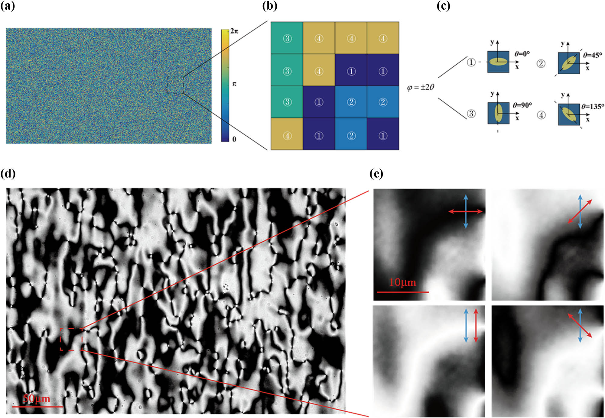
Figure 1.Design of LC metasurface diffuser. (a) Designed phase distribution of the LC metasurface diffuser. (b) Local phase distribution of the LC metasurface diffuser with the four-order phase. (c) The four LCMs with different rotation angles corresponding to the four-order phase distribution. (d) The POM image of the metasurface diffuser. (e) The local magnification POM images under different polarization states, and the blue and red arrows denote the input and output polarization states of light.

B. Multiple-Dimensional PSFs through a Single Diffuser

The functionalities and performances of an imaging system can be quantified by calculating its PSF. Our crucial intuition is to build a diffuser whose PSFs change with chirality, wavelengths, and position so that the associated information can be recorded into a snapshot speckle, and the polarization, spectral, and spatial information can be recovered through the conventional deconvolution technique, shown in Fig. 2. Suppose an object point is at a distance of $z_{1}$ from the diffuser. The optical field passes through the diffuser resulting in phase changes. Subsequently, the field propagates to the sensor at the distance $z_{2}$ , resulting in the PSF $P_{λ, σ, z}$ , which is the squared magnitude of the complex wave field at the sensor plane [42]: $P_{λ, σ, z} = {| F {A \cdot \exp [i (Φ_{obj} + Φ_{LC} + Φ_{sensor})]} |}^{2},$ (4)where $F$ represents the Fourier transform, $A$ is the amplitude of the point source, and $Φ_{{obj / LC / sensor}}$ are the phase delays induced by propagating the object to the LC metasurface diffuser $Φ_{obj} = k (z_{1} + \frac{x^{2} + y^{2}}{2 z_{1}})$ , the diffuser itself $Φ_{LC} = 2 σ θ$ , and propagating from the LC metasurface diffuser to the sensor $Φ_{sensor} = k (z_{2} + \frac{x^{2} + y^{2}}{2 z_{2}})$ . $k$ is the wavenumber $2 π / λ$ , $σ$ is the chirality $\pm 1$ , and $θ$ is the orientation angle of LCM. Equation (4) shows that the PSF generated by the diffusion and diffraction of an LC metasurface diffuser depends on the spatial distribution $(x, y, z)$ , wavelength $(λ)$ , and chirality $(σ)$ of an object point (see Appendix B for details). These phase terms are summed up at k-space and converted to the spatial domain through Fourier transform. Therefore, this multiple-dimensional information can be reconstructed from PSF analysis in a single image, shown in Figs. 2(c) and 2(d). Information in the ( $x, y$ ) plane can be recovered by deconvolution based on the shift-invariance of PSFs. Information recovery in ( $z, λ, σ$ ) spaces relies on the axial-spectral-polarization dependency of the diffuser.

Figure 2.Schematic of the spatial–spectral–polarization meta-optical imaging system. (a) Light from two multispectral objects with different spatial and polarization (left, left-circularly polarized; right, right-circularly polarized) information propagating through the designed LC metasurface diffuser generates a speckle pattern on a monochromatic camera. (b) Speckle patterns produced by two-point objects with respective spatial and polarization information of the two multi-dimensional objects, taken as corresponding multi-dimensional PSFs. (c) Reconstructed multi-dimensional images from the monochromatic speckle images using corresponding PSFs. (d) The recovered image of the two objects by superimposing individual reconstructed images.

C. Image Formation and Recovery

Our Snapshot 5D Imaging system is mainly based on Fresnel diffraction and Fourier optics [43], and for an incoherent imaging system, it is described as $I (x, y, z, λ, σ) = O (x, y, z, λ, σ) * PSF (x, y, z, λ, σ),$ (5)where $*$ denotes convolution and $PSF (x, y, z, λ, σ)$ is the PSF. $O (x, y, z, λ, σ)$ and $I (x, y, z, λ, σ)$ are the objects and the images (also called the input and output signals). $(x, y, z)$ is the spatial distribution of an object, and $λ$ and $σ$ are the wavelength and chirality of the incident light. As the description in Section 2.B, in the memory effect range, the shift-invariance PSFs are axial–spectral–polarization dependent, making PSFs uncorrelated under different spatial–spectral–polarization conditions. It can be given by $PSF (z_{1}, λ_{1}, σ_{1}) ⋆ PSF (z_{2}, λ_{2}, σ_{2}) \approx {\begin{matrix} 0, & if | z_{1} - z_{2} | > T_{z} \lor | λ_{1} - λ_{2} | > T_{λ} \lor σ_{1} \neq σ_{2} \\ δ, & if | z_{1} - z_{2} | < T_{z} \land | λ_{1} - λ_{2} | < T_{λ} \land σ_{1} = σ_{2} \end{matrix},$ (6)where $⋆$ denotes the correlation operator, and $δ$ denotes the impulse response function. $T$ represents the response threshold value of each dimension. The variation of $z$ and $λ$ will lead to additional phase delays $Φ_{Δ z} = k (Δ z + \frac{x^{2} + y^{2}}{2 z} \cdot \frac{Δ z}{z + Δ z})$ and $Φ_{Δ λ} = k \cdot \frac{Δ λ}{λ + Δ λ} \cdot r$ , which changes the intensity profile on the detector, decreasing the correlation between PSFs. The polarization selective properties described as in Eq. (3) explain the different phase delay assigned to LCP and RCP incidences, providing significant difference among PSFs.

The speckle pattern with all the spatial distribution, wavelength, and chirality information of the object is the composite response of the LC metasurface diffuser. It can be expressed as $I = \sum_{x, y, z, λ, σ} I (x, y, z, λ, σ) = \sum_{x, y, z, λ, σ} [O (x, y, z, λ, σ) * PSF (x, y, z, λ, σ)] .$ (7)

Therefore, the object with interesting spatial–spectral–polarization information can be reconstructed from the image overlapping diverse factors by deconvoluting PSF with respect 5D property as follows: $O (x_{0}, y_{0}, z_{0}, λ_{0}, σ_{0}) = deconv [I, PSF (x_{0}, y_{0}, z_{0}, λ_{0}, σ_{0})] .$ (8)

D. Deconvolution Algorithm

We use Wiener deconvolution for image reconstruction, and it is expressed as follows [44]: $O (x_{0}, y_{0}, z_{0}, λ_{0}, σ_{0}) = deconv [I, PSF (x_{0}, y_{0}, z_{0}, λ_{0}, σ_{0})] = {FFT}^{- 1} {\frac{FFT (I) \cdot FFT {[PSF (x_{0}, y_{0}, z_{0}, λ_{0})]}^{c}}{{| FFT [PSF (x_{0}, y_{0}, z_{0}, λ_{0}, σ_{0})] |}^{2} + SNR (f)}},$ (9)where $FFT (\cdot)$ and ${FFT}^{- 1} (\cdot)$ denote the Fourier transform and its inverse, respectively. ${(\cdot)}^{c}$ is the complex conjugate and $SNR (f)$ is the signal-to-noise ratio. Using the spatial–spectral–polarization-dependent behavior of the LC metasurface diffuser described in Eq. (6), we can reconstruct the object of interest with high quality.

3. EXPERIMENT

A. Spatial Resolution

As an imaging system, the spatial resolution of MCI is measured first. The setup of MCI is shown in Fig. 3(a). A projector (Acer X118H) is used to generate object patterns. The magnification lens of the projector is removed, and an iris is set to filter out background light from the projector. The LC metasurface diffuser then modulates the light that comes from the projector, and a monochromatic camera (Daheng, MER-500-7UM) is used to capture the intensity profile. The exposure time to capture PSFs was set to 80 ms, and that to capture objects was set to 16 ms. The distance from the object patterns to the metasurface is 15 cm, and the camera is placed 2 cm behind the metasurface. To decide the resolution of this system, resolution chart patterns with different gaps, shown in Fig. 3(c), are loaded on the center area of the projector. The recovered images and their profiles are shown in Fig. 3(d), illustrating that the spatial resolution of this system is around 28 μm, as the peak–valley ratio is about 1.52 at this scale. The deconvolution algorithm takes 0.43 s to reconstruct information from the PSF and the corresponding speckle pattern pair. The axial resolution and spectral resolution are discussed in Appendix A, and more experimental results are exhibited in Appendix C.

Figure 3.Spatial resolution of the MCI system. (a) Schematic diagram of the experimental setup. (b) The diagonal length of the DMD chip used in the projector is 0.55 in., and the pixel size is 14 μm. (c) The resolution chart loaded on the projector and the recovered images. The gaps of each line are 1, 2, and 3 pixels, respectively. (d) Intensity profile of lines in (c). Scale bar: 50 μm in (c).

B. Multispectral Imaging

The same setup shown in Fig. 3(a) is used to generate object patterns for multispectral imaging of MCI. By loading different patterns with different RGB values, objects’ spatial and spectral information could be changed conveniently. In practice, seven different capital letters with different colors are projected respectively. The speckle patterns captured by the camera are shown in Fig. 4(a) (Pseudocolore is applied for convenient exhibition). Then, a single central pixel with the aforesaid colors is lightened up respectively, and the captured speckles are taken as multispectral PSFs of MCI, as shown in Fig. 4(b). The reconstructed multispectral images are finally obtained by deconvolving different spectral PSFs with different speckle patterns, exhibited in Fig. 4(c). The ground truth patterns loaded on the projector are shown in Fig. 4(d). As expected, each speckle pattern is smoothly reconstructed. Figure 4(e) demonstrates the composite multispectral image superimposing with seven individual spectral images of Fig. 4(c).

Figure 4.Schematic of MCI’s multispectral imaging. (a) The raw speckle patterns generated by different chromatic objects. (b) The PSFs generated by a central point object with corresponding colors. (c) The images reconstructed from the speckle patterns using corresponding PSFs. (d) The ground truth pictures projected on the projector, which are projected respectively. (e) The full reconstructed image by superimposing seven individual spectral images in (c). Scale bar: 1000 μm in speckle patterns and PSFs, and 100 μm in reconstructed images.

C. Polarization Imaging

For verifying the polarization selective ability of MCI, we leverage the setup shown in Figs. 5(a) and 5(b). Different from the setup in Fig. 3, two pairs of the polarizer and the quarter-wave plate were employed. The first pair of the polarizer and quarter-wave plate translates the incident light into CP light. By rotating the quarter-wave plate, LCP light or RCP light can be generated. Then the CP light transmits through the metasurface diffuser and converts incident CP light to the opposite chirality. The LC metasurface diffuser can obtain a high polarization conversion efficiency ( $> 95 %$ ) at the designed wavelength, which is about 532 nm, but the efficiency will decrease away from that wavelength. So the second pair of the polarizer and the quarter-wave plate is applied to filter out the co-polarized light remaining in transmitted light. In the experiment, two letters, “H” and “E,” with the same color, were loaded on the projector. Figure 5(c) shows the raw speckle patterns captured by the camera. The rotation arrows in the upper left indicate the polarization of each pattern (blue for RCP, red for LCP). Figure 5(d) shows the PSFs with different polarizations. Figures 5(e) and 5(f) show the reconstructed images by deconvolving the different polarization speckle patterns with different polarization PSFs. There are two rotation arrows in the upper left. The first indicates the polarization of the speckle pattern, and the second indicates the polarization of the PSF used for deconvolving [e.g., the upper picture in Fig. 5(f) has two arrows, blue on the left and red on the right, indicating this picture is the result of the RCP speckle pattern deconvolving with the LCP PSF]. According to these experimental observations, MCI shows high sensitivity to the polarization of incident objects, and objects can be recovered only when the speckle patterns and PSFs are at the same polarization.

Figure 5.Schematic of MCI’s polarization selective characterization. (a) Schematic diagram of the experimental setup. The first pair of the polarizer and quarter-wave plate converts incident light to LCP light (indicated by the red rotation spinning arrow). Then the LCP light transmits through the metasurface and is converted to RCP light (indicated by the blue rotation spinning arrow). Limited by the polarization conversion efficiency of the metasurface, some LCP light is left in transmitted light. The second pair of the polarizer and the quarter-wave plate is employed to remove LCP light. (b) has the same experimental setup as (a), except the rotation angle of two quarter-wave plates is changed for the generation and removal of RCP light. (c) The raw speckle patterns with different polarization (blue for RCP, red for LCP). (d) The PSFs with different polarization. (e) The reconstructed images from the speckle patterns by deconvolution with PSFs of the same polarization. (f) The reconstructed images from the speckle patterns by deconvolution with PSFs of the orthogonal polarization (there are two rotation spinning arrows in the upper left; the left and right arrows indicate polarization of speckle pattern and PSF). Scale bar: 1000 μm in speckle patterns and PSFs, and 100 μm in reconstructed images.

D. 5D Imaging

To evaluate the performance of our MCI in spatial–spectral–polarization 5D $(x, y, z, λ, σ)$ imaging, two objects with different 5D properties are projected and superimposed on the sensor. The experimental setup is shown in Fig. 6(a). The two patterns with different colors are loaded on the left and right areas of the projector. After transmitting through a diaphragm and a polarizer, the beam from the projector becomes polarized light. The left part of the beam is reflected by a mirror to another path. Beams in two paths are polarized into orthogonal circular polarizations while transmitting through quarter-wave plates with different fast axis orientations. Then two beams are superimposed by a beam combiner and modulated by the metasurface diffuser. Finally, the raw speckle pattern is recorded by a camera, shown in Fig. 6(b). Before recovering the actual pattern, a two-point source with different colors was loaded on the projector to generate corresponding 5D PSFs respectively, shown in the upper part of Figs. 6(c) and 6(d). The reconstructed images obtained by deconvolving the PSFs with speckle patterns in Fig. 6(b) were exhibited in the lower parts of Figs. 6(c) and 6(d). The experimental results shown above illustrate that the two objects with different 5D information can be reconstructed from the overlapped speckle pattern. PSFs with different 5D information can retrieve different objects in the superimposed speckle pattern. Note that the quality of reconstructed images in Figs. 6(c) and 6(d) is not as good as shown in Figs. 4(c) and 5(e), which is likely due to the polarization conversion efficiency of our metasurface diffuser. Although the metasurface converts polarization of incident light into the opposite handedness, some co-polarized light remains in transmitted light, causing minor deterioration for recognizing objects with orthogonal polarization.

Figure 6.Schematic of MCI’s 5D imaging. (a) Schematic diagram of the experimental setup. Two objects (left and right) are projected simultaneously and transmitted through a diaphragm and polarizer, which blocks stray light and converts to linear polarization. M1, M2, and M3 are mirrors, and M1 and M2 reflect the left object to another path. Quarter-wave plates circularly polarize both objects. The two quarter-wave plates are set to orthogonal rotation angles to produce different circularly polarized objects. Following M3 reflects the left object to the main path and the beam splitter superimposes both objects together. Then the superimposed beam transmits through the metasurface and is recorded by the camera. (b) The superimposed speckle pattern of two objects with different 5D information. (c) The individual measured PSF of the right path and the reconstructed image from the superimposed speckle pattern by deconvolution. (d) The individual measured PSF of the left path and the reconstructed image from the superimposed speckle pattern by deconvolution. Scale bar: 1000 μm in speckle patterns and PSFs, and 100 μm in reconstructed images.

4. CONCLUSION

We demonstrate a lensless snapshot 5D imaging system by employing a computational technique and the metasurface’s spatial–spectral–polarization sensitivity. The 5D information of the object is encoded by the metasurface as speckle patterns, which allow us to apply a deconvolution algorithm to reconstruct the 5D information of interest by corresponding PSFs. Our demonstrations present a compact and inexpensive technique for snapshot 5D imaging that might be promising for material classification and identification, biomedicine, and industry applications. As a general framework of imaging and detection, our proposal is promising to promote the next generation of engineering optics [45,46].

Acknowledgment

Acknowledgment. Y. Lei thanks Dr. Dongliang Tang for his help in LC metasurface fabrication and experimental design.

APPENDIX A: CONTRAST RANDOM PHASE PROFILE WITH FOCUS PHASE PROFILE IN THE ALGORITHM’S PERFORMANCE

J I (A, B) = \frac{| A \cap B |}{| A \cup B |},

Figure 7.Wavelength resolution comparison of random and focus phase profiles. We simulate the imaging results under these two phase profiles with a center wavelength of 532 nm and deconvolve these images with their PSFs of varying wavelengths. (a) and (c) are the reconstructed results under different PSFs with corresponding phase profiles at different wavelengths. (b) and (d) show the simulated PSFs for each phase profile. (e) The Jaccard index of the reconstructed results compared with the ground truth image. (f) The Pearson correlation coefficient of the reconstructed results compared with the ground truth image.

Figure 8.Spatial resolution comparison of random and focus phase profiles. We simulate the imaging results under these two phase profiles at the distance of 15 cm along the $z$ axis and deconvolve these images with their PSFs varying the distance along the $z$ axis. (a) and (c) are the reconstructed results under different PSFs at different depths with corresponding phase profiles. (b) and (d) show the simulated PSFs for each phase profile. (e) The Jaccard index of the reconstructed results compared with the ground truth image. (f) The Pearson correlation coefficient of the reconstructed results compared with the ground truth image.

2 \times

APPENDIX B: ANALYSIS OF SPATIAL–SPECTRAL–POLARIZATION DEPENDENCY OF LC METASURFACE DIFFUSER

Figures 9 and 10 present a simulation example for the PSF of our LC metasurface diffuser by varying the object’s spatial axial location, wavelength, and chirality of incidence and calculating the PCC for each PSF. PSFs change with the spatial-spectral-polarization factors and the PCC between PSFs is a significant indicator to help us judge whether the deconvolution algorithm might reconstruct the information we need.

Figure 9.For LCP incidence, the Pearson correlation coefficients between PSFs with different object depths and wavelengths of incidence.

Figure 10.For RCP incidence, the Pearson correlation coefficients between PSFs with different object depths and wavelengths of incidence.

APPENDIX C: EXPERIMENT OF AXIAL PSF DEPENDENCY AND AXIAL RESOLUTION MEASUREMENT

To verify the simulation results of Appendices A and B, as an example, we calculated the dependency of axial PSFs and valued axial resolution. Figure 11 (a) shows the experiment setup. PSFs of different axial distances are recorded first. Then two objects are loaded on the projector at a different distance from the diffuser, and the distance between the two object planes is 10 mm. The camera recorded images respectively and added two images together. The deconvolution algorithm with different PSFs is then applied to this image with two objects. The reconstructed results and the according PSFs are shown in Figs. 11 (b) and 11 (c). The Pearson correlation coefficient between reconstructed images with different axial distances is plotted in Fig. 11 (d). Experiment results illustrate that the axial resolution is better than 10 mm, and the axial dependency of the LC metasurface diffuser is demonstrated.

Figure 11.Axial resolution experimental result. (a) Scheme of $z$ -direction resolution measurement. Two objects with different distances from the diffuser are imaged respectively, and two images are added together as the pattern to recover. (b) Different PSFs measured from different distances and corresponding reconstructed images. (c) The Pearson correlation coefficient of the reconstructed results compared with the image of the original location. Scale bar: 1000 μm in PSFs and 100 μm in reconstructed images.

APPENDIX D: MEMORY EFFECT OF MCI SYSTEM

\pm 6 mm

Figure 12.Test of memory effect range. (a) Scheme of memory effect range measurement. Objects are shifting out of the original position along with the projector moving, and the moving step is 0.5 mm. (b) Reconstructed images of objects in different positions. (c)–(h) Enlarged images of (b). Scale bar: 100 μm.

Fabrication Process

LC metasurfaces were fabricated using a DMD exposure system and the fabrication process is kept in a dust-free environment to obtain high-quality samples. Photoalignment materials we used in the fabrication are dimethylformamide (DMF) and sulfonated azo dye (SD1), mixed with a ratio of 99.5:0.5. First, the glass substrate was washed by ultrasonic cleaning, adequately heated, UV-light exposed, and compressed air blown. Second, the mixed solution of DMF and SD1 was dropped uniformly on the constant rotating glass substrate to form an evenly distributed orientation layer. Third, the samples were exposed by a DMD to achieve the expected rotation angles of the LC molecules. Fourth, a solution of LC materials consisting of RM257 (14%), Irgacure184 (1%), and methylbenzene (85%) was dropped on an orientation layer and rotated uniformly. Finally, the LC metasurfaces were completed after solidification within the unpolarized light with a wavelength of 365 nm.

References

[1] B. Javidi, X. Shen, A. S. Markman, P. Latorre-Carmona, A. Martinez-Uso, J. M. Sotoca, F. Pla, M. Martinez-Corral, G. Saavedra, Y.-P. Huang. Multidimensional optical sensing and imaging system (MOSIS): from macroscales to microscales. Proc. IEEE, 105, 850-875(2017).

[2] B. Javidi, S.-H. Hong, O. Matoba. Multidimensional optical sensor and imaging system. Appl. Opt., 45, 2986-2994(2006).

[3] Y. Zheng, M.-J. Sun, Z.-G. Wang, D. Faccio. Computational 4D imaging of light-in-flight with relativistic effects. Photonics Res., 8, 1072-1078(2020).

[4] Y.-Q. Zhao, L. Zhang, D. Zhang, Q. Pan. Object separation by polarimetric and spectral imagery fusion. Comput. Vis. Image Underst., 113, 855-866(2009).

[5] I. M. Vellekoop, A. Lagendijk, A. Mosk. Exploiting disorder for perfect focusing. Nat. Photonics, 4, 320-322(2010).

[6] W. Gong, S. Han. Experimental investigation of the quality of lensless super-resolution ghost imaging via sparsity constraints. Phys. Lett. A, 376, 1519-1522(2012).

[7] A. K. Singh, D. N. Naik, G. Pedrini, M. Takeda, W. Osten. Exploiting scattering media for exploring 3D objects. Light Sci. Appl., 6, e16219(2017).

[8] N. Antipa, G. Kuo, R. Heckel, B. Mildenhall, E. Bostan, R. Ng, L. Waller. DiffuserCam: lensless single-exposure 3D imaging. Optica, 5, 1-9(2018).

[9] S. K. Sahoo, D. Tang, C. Dang. Single-shot multispectral imaging with a monochromatic camera. Optica, 4, 1209-1213(2017).

[10] K. Monakhova, K. Yanny, N. Aggarwal, L. Waller. Spectral DiffuserCam: lensless snapshot hyperspectral imaging with a spectral filter array. Optica, 7, 1298-1307(2020).

[11] A. Goetschy, A. Stone. Filtering random matrices: the effect of incomplete channel control in multiple scattering. Phys. Rev. Lett., 111, 063901(2013).

[12] I. M. Vellekoop, A. Mosk. Focusing coherent light through opaque strongly scattering media. Opt. Lett., 32, 2309-2311(2007).

[13] G. Li, S. Chen, N. Pholchai, B. Reineke, P. W. H. Wong, E. Y. B. Pun, K. W. Cheah, T. Zentgraf, S. Zhang. Continuous control of the nonlinearity phase for harmonic generations. Nat. Mater., 14, 607-612(2015).

[14] J. Li, Y. Wang, C. Chen, R. Fu, Z. Zhou, Z. Li, G. Zheng, S. Yu, C. W. Qiu, S. Zhang. From lingering to rift: metasurface decoupling for near-and far-field functionalization. Adv. Mater., 33, 2007507(2021).

[15] Y. Guo, S. Zhang, M. Pu, Q. He, J. Jin, M. Xu, Y. Zhang, P. Gao, X. Luo. Spin-decoupled metasurface for simultaneous detection of spin and orbital angular momenta via momentum transformation. Light Sci. Appl., 10, 1(2021).

[16] Q. Fan, W. Xu, X. Hu, W. Zhu, T. Yue, C. Zhang, F. Yan, L. Chen, H. J. Lezec, Y. Lu. Trilobite-inspired neural nanophotonic light-field camera with extreme depth-of-field. Nat. Commun., 13, 2130(2022).

[17] F. Zhang, Y. Guo, M. Pu, X. Li, X. Ma, X. Luo. Metasurfaces enabled by asymmetric photonic spin-orbit interactions. Opto-Electron. Eng., 47, 200366(2020).

[18] Z.-B. Fan, Z.-K. Shao, M.-Y. Xie, X.-N. Pang, W.-S. Ruan, F.-L. Zhao, Y.-J. Chen, S.-Y. Yu, J.-W. Dong. Silicon nitride metalenses for close-to-one numerical aperture and wide-angle visible imaging. Phys. Rev. Appl., 10, 014005(2018).

[19] Z.-B. Fan, H.-Y. Qiu, H.-L. Zhang, X.-N. Pang, L.-D. Zhou, L. Liu, H. Ren, Q.-H. Wang, J.-W. Dong. A broadband achromatic metalens array for integral imaging in the visible. Light Sci. Appl., 8, 67(2019).

[20] C. Fang, Q. Yang, Q. Yuan, X. Gan, J. Zhao, Y. Shao, Y. Liu, G. Han, Y. Hao. High-Q resonances governed by the quasi-bound states in the continuum in all-dielectric metasurfaces(2022).

[21] X. Zou, Y. Zhang, R. Lin, G. Gong, S. Wang, S. Zhu, Z. Wang. Pixel-level Bayer-type colour router based on metasurfaces. Nat. Commun., 13, 3288(2022).

[22] Z.-L. Deng, Y. Cao, X. Li, G. P. Wang. Multifunctional metasurface: from extraordinary optical transmission to extraordinary optical diffraction in a single structure. Photonics Res., 6, 443-450(2018).

[23] J. Liu, M. Shi, Z. Chen, S. Wang, Z. Wang, S. Zhu. Quantum photonics based on metasurfaces. Opto-Electron. Adv., 4, 09200092(2021).

[24] H. Gao, X. Fan, W. Xiong, M. Hong. Recent advances in optical dynamic meta-holography. Opto-Electron. Adv., 4, 210030(2021).

[25] S. Colburn, A. Majumdar. Metasurface generation of paired accelerating and rotating optical beams for passive ranging and scene reconstruction. ACS Photonics, 7, 1529-1536(2020).

[26] F. Zhao, Z. Shen, D. Wang, B. Xu, X. Chen, Y. Yang. Synthetic aperture metalens. Photonics Res., 9, 2388-2397(2021).

[27] E. Arbabi, S. M. Kamali, A. Arbabi, A. Faraon. Full-Stokes imaging polarimetry using dielectric metasurfaces. ACS Photonics, 5, 3132-3140(2018).

[28] N. A. Rubin, G. D’Aversa, P. Chevalier, Z. Shi, W. T. Chen, F. Capasso. Matrix Fourier optics enables a compact full-Stokes polarization camera. Science, 365, eaax1839(2019).

[29] F. Zhao, R. Lu, X. Chen, C. Jin, S. Chen, Z. Shen, C. Zhang, Y. Yang. Metalens-assisted system for underwater imaging. Laser Photonics Rev., 15, 2100097(2021).

[30] F. Zhang, M. Pu, X. Li, X. Ma, Y. Guo, P. Gao, H. Yu, M. Gu, X. Luo. Extreme-angle silicon infrared optics enabled by streamlined surfaces. Adv. Mater., 33, 2008157(2021).

[31] M. Jang, Y. Horie, A. Shibukawa, J. Brake, Y. Liu, S. M. Kamali, A. Arbabi, H. Ruan, A. Faraon, C. Yang. Wavefront shaping with disorder-engineered metasurfaces. Nat. Photonics, 12, 84-90(2018).

[32] H. Kwon, E. Arbabi, S. M. Kamali, M. Faraji-Dana, A. Faraon. Computational complex optical field imaging using a designed metasurface diffuser. Optica, 5, 924-931(2018).

[33] X. Hua, Y. Wang, S. Wang, X. Zou, Y. Zhou, L. Li, F. Yan, X. Cao, S. Xiao, D. P. Tsai. Ultra-compact snapshot spectral light-field imaging. Nat. Commun., 13, 2732(2022).

[34] D. Tang, Z. Shao, Y. Zhou, Y. Lei, L. Chen, J. Xie, X. Zhang, X. Xie, F. Fan, L. Liao. Simultaneous surface display and holography enabled by flat liquid crystal elements. Laser Photonics Rev., 16, 2100491(2022).

[35] Q. Xu, T. Sun, C. Wang. Coded liquid crystal metasurface for achromatic imaging in the broadband wavelength range. ACS Appl. Nano Mater., 4, 5068-5075(2021).

[36] X. Lu, X. Li, Y. Guo, M. Pu, J. Wang, Y. Zhang, X. Li, X. Ma, X. Luo. Broadband high-efficiency polymerized liquid crystal metasurfaces with spin-multiplexed functionalities in the visible. Photonics Res., 10, 1380-1393(2022).

[37] Y. Ji, F. Fan, Z. Zhang, Z. Tan, X. Zhang, Y. Yuan, J. Cheng, S. Chang. Active terahertz spin state and optical chirality in liquid crystal chiral metasurface. Phys. Rev. Mater., 5, 085201(2021).

[38] S. Zhou, Z. Shen, X. Li, S. Ge, Y. Lu, W. Hu. Liquid crystal integrated metalens with dynamic focusing property. Opt. Lett., 45, 4324-4327(2020).

[39] J. Li, P. Yu, S. Zhang, N. Liu. Electrically-controlled digital metasurface device for light projection displays. Nat. Commun., 11, 1(2020).

[40] M. V. Berry. The adiabatic phase and Pancharatnam’s phase for polarized light. J. Mod. Opt., 34, 1401-1407(1987).

[41] S. Pancharatnam. Generalized theory of interference and its applications. Proceedings of the Indian Academy of Sciences-Section A, 398-417(1956).

[42] H. Xu, H. Hu, S. Chen, Z. Xu, Q. Li, T. Jiang, Y. Chen. Hyperspectral image reconstruction based on the fusion of diffracted rotation blurred and clear images. Opt. Lasers Eng., 160, 107274(2023).

[43] J. W. Goodman. Introduction to Fourier Optics(2005).

[44] S. Quirin, R. Piestun. Depth estimation and image recovery using broadband, incoherent illumination with engineered point spread functions. Appl. Opt., 52, A367-A376(2013).

[45] X. Luo. Subwavelength optical engineering with metasurface waves. Adv. Opt. Mater., 6, 1701201(2018).

[46] X. Luo. Subwavelength artificial structures: opening a new era for engineering optics. Adv. Mater., 31, 1804680(2019).