
Yufang Cai, Taoyan Chen, Jue Wang, Gongjie Yao. Image Noise Reduction in Computed Tomography with Non-Local Means Algorithm Based on Adaptive Filtering Coefficients[J]. Acta Optica Sinica, 2020, 40(7): 0710001
- Acta Optica Sinica
- Vol. 40, Issue 7, 0710001 (2020)
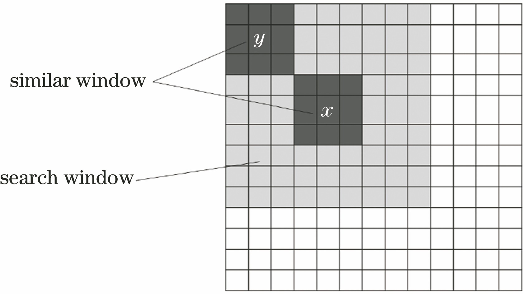
Fig. 1. Relationship diagram of similar window and search window of NLM algorithm
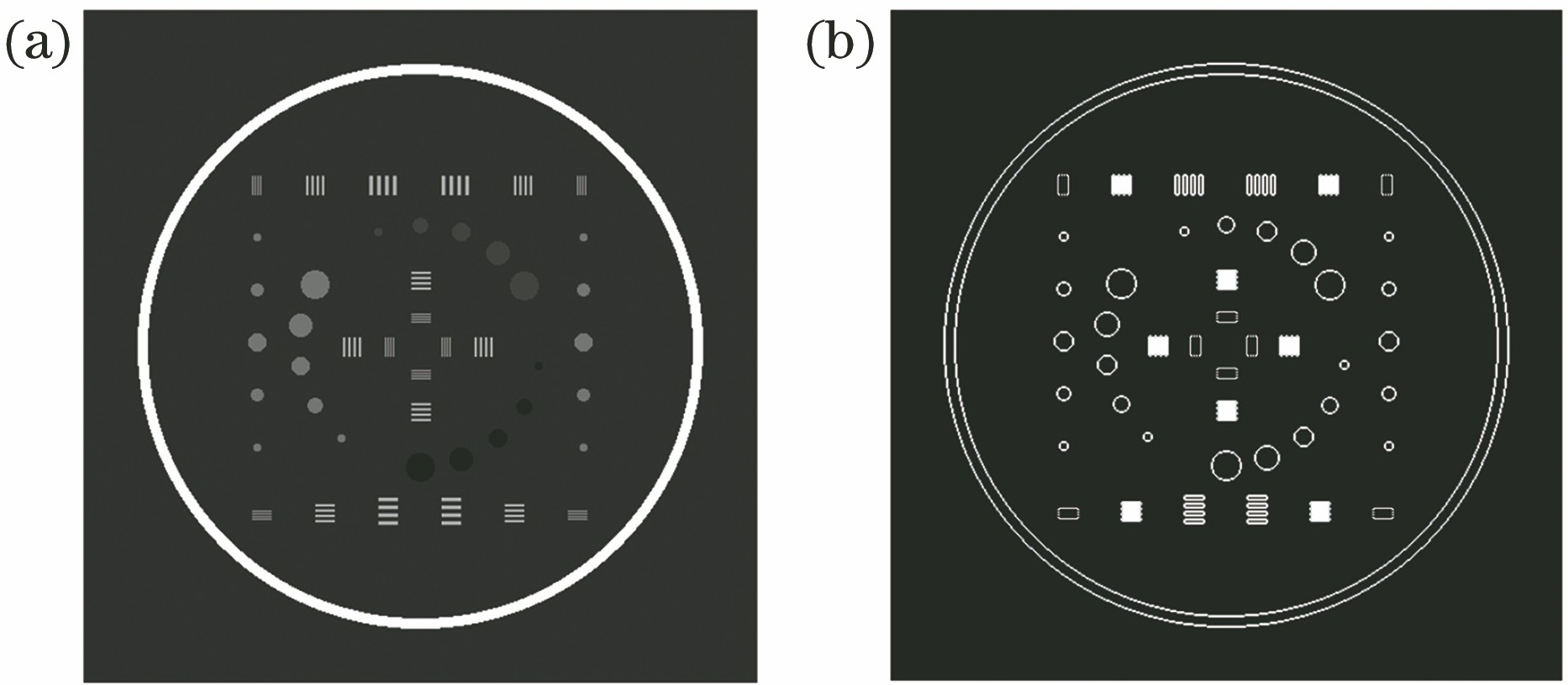
Fig. 2. Structural tensor decomposition. (a) Original image; (b) schematic of structure tensor
Fig. 3. Flowchart of ST-NLM algorithm
Fig. 4. Gaussian noise simulated image and local magnification of filtering results at different noise levels. (a) Simulated image; (b) σ=1; (c) σ=4; (d) σ=5; (e) σ=12
Fig. 5. CT image of spatial resolution testing card. (a) Original image; (b) NLM; (c) method in Ref. [12]; (d) ST-NLM
Fig. 6. Gray curves obtained by different filtering methods
Fig. 7. Typical CT slices of insect 1. (a) Original image; (b) locally enlarged image; (c) NLM; (d) method in Ref. [12]; (e) ST-NLM
Fig. 8. CT image of the 520th slice of insect 1. (a) Original image; (b) locally enlarged image; (c) NLM; (d) method in Ref. [12]; (e) ST-NLM
Fig. 9. CT image of the 434th slice of insect 2. (a) Original image; (b) locally enlarged image; (c) NLM; (d) method in Ref. [12]; (e) ST-NLM
|
Table 1. Quantitative evaluation of SSIM and PSNR by different methods
|
Table 2. CT system parameters for experiment
|
Table 3. Experimental parameters of different images
|
Table 4. Index of image sharpness
|
Table 5. Comparison of operating time among various filtering algorithmss

Set citation alerts for the article
Please enter your email address
© Copyright 2018-2021 | Chinese Laser Press. All Rights Reserved 沪ICP备15018463号-20