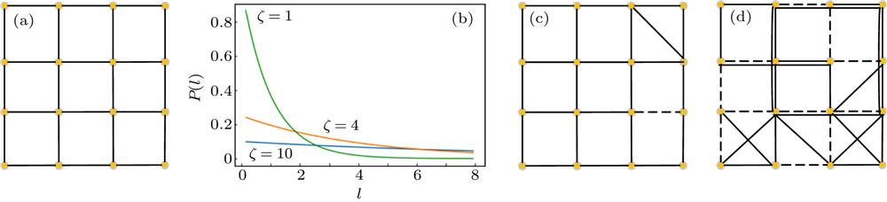
Fig. 1. The connection of nodes within the layer in small networks. The solid line represents the actual connection while the dotted line denotes the lattice line. The parameters are 〈k〉 = 3, N = 16. (a) The connection between nodes defined in the previous papers. (b) The exponential distribution of l: P(l) ∼ exp(–l/ζ), ζ = 1, 4, 10. (c) The distance l between nodes obeys the exponential distribution: P(l) ∼ exp(–l/0.1). (d) The distance l between nodes obeys the exponential distribution: P(l) ∼ exp(–l/10).

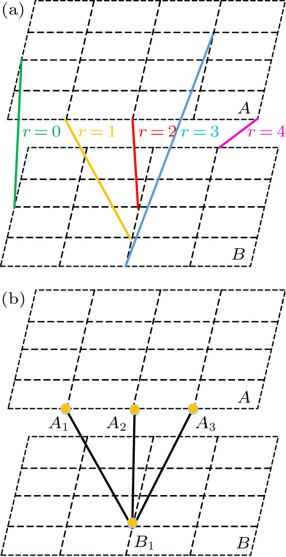
Fig. 2. (a) The connections between layers in a two-layer network when r = 0, 1, 2, 3, 4 separately. (b) A node in one layer connects to more than one node in other layers. When r = 1, node B₁ is connected to the nodes of A₁, A₂, A₃.

Fig. 3. Load distribution process. The parameters are a = 1/3, b = 1/2, c = 1, N = 9. The valid nodes are marked in yellow and the disabled ones are depicted in red. When t = 0, the initial loads of nodes are L₁(0) = 1/6, L₂(0) = 3/6, L₃(0) = 1/6, L₄(0) = 1/6, L₅(0) = 3/6, L₆(0) = 2/6, L₇(0) = 0, L₈(0) = 1/6, L₉(0) = 0. Since node 5 is invalid, its load will distribute to nodes 2, 4, 6 according to the load distribution strategy. When t = 1, the loads of nodes 2, 4, 6 become L₂(1) = 3/4, L₄(1) = 1/4, L₆(1) = 1/2. Owing to L₂(1) > c × C₂, node 2 becomes ineffective and will distribute its load to nodes 1, 3. Other nodes will not change their state due to L_i(1) < c × C_i, i = 1, 3, 4, 6, 7, 8, 9. When t = 2, nodes 1, 3 become invalid because their loads exceed their capacities (L₁(2) > c × C₁, L₃(2) > c × C₃).

Fig. 4. Cascading failure processes of two models in double-layer spatial networks in the first iteration. The parameters are a = 0.25, b = 2, c = 1.5, r = 1, ζ = 0.2, p = 0.25, N₁ = N₂ = 4, 〈k〉₁ = 〈k〉₂ = 1. N_x and 〈k〉_x are the number of nodes and average degree of layer x individually, x = 1.2. In layer x, the number of nodes initially removed is N_x × p = 1. (a) The cascading failure process of the first model. In Step 1, nodes A₂ and B₂ are initially removed. In Step 2, node B₄ fails due to overload (13/24 = c × C_B4 < L_B4(1) = 2/3). In Step 3 (effect 1), node B₄ recovers because A₁ is valid. In Step 4, A₄ and B₄ become invalid owing to the percolation process. (b) The cascading failure process of the second model. The behaviors of nodes are consistent with (a) in Step 1 and Step 2. In Step 3 (effect 2), node A₁ becomes invalid because B₄ is invalid. In Step 4, node A₄ fails owing to the percolation process.

Fig. 5. (a) Entropy E as a function of ζ on the spatial network. The parameters are N = 900, 〈k〉 = 4. (b) Entropy E as a function of ln N on the spatial network, regular network, ER network, and BA network separately. The parameters are ζ = 0.2, 〈k〉 = 4. Each point on the above figures is the average value of 20 experiments.

Fig. 6. The evolution processes of two double-layer spatial networks under effect 1 and effect 2 when p = 0.2. The parameters are a = 5, b = 0.8, c = 0.5, r = 1, ζ = 0.2, N₁ = N₂ = 900, 〈k〉₁ = 〈k〉₂ = 4. N_x and 〈k〉_x are the number of nodes and average degree of layer x individually, x = 1, 2. Each point on the figures is the average value of 20 experiments. Panels (a) and (b) are the changes of dynamic network size S(t) and dynamic network entropy E(t) under effect 1. Panel (c) reveals the nodes state when the network is stable under effect 1. Panels (d)–(f) are similar to panels (a)–(c) but under effect 2.

Fig. 7. The evolution processes of two double-layer spatial networks under effect 1 and effect 2 when p = 0.7. The parameters are a = 5, b = 0.8, c = 0.5, r = 1, ζ = 0.2, N₁ = N₂ = 900, 〈k〉₁ = 〈k〉₂ = 4. N_x and 〈k〉_x are the number of nodes and average degree of layer x individually, x = 1, 2. Each point on the figures is the average value of 20 experiments. Panels (a) and (b) are the changes of dynamic network size S(t) and dynamic network entropy E(t) under effect 1. Panel (c) shows the nodes state when the network is stable under effect 1. Panels (d)–(f) are similar to panels (a)–(c) but under effect 2.

Fig. 8. The changes of S under the effect of ζ in multilayer spatial networks. When p is small, as ζ decreases, the network robustness becomes more reliable. When p is large, the network performs better as ζ increases. Each point on the figures is the average value of 20 experiments. (a) Two-layer networks. The parameters are a = 6, b = 0.5, c = 1.5, r = 3, N₁ = 225, N₂ = 400, 〈k〉₁ = 5, 〈k〉₂ = 6. N_x and 〈k〉_x are the number of nodes and average degree of layer x individually, x = 1.2. (b) Three-layer networks. The added parameters are N₃ = 625 and 〈k〉₃ = 7. (c) Four-layer networks. The added parameters are N₄ = 900 and 〈k〉₄ = 8.

Fig. 9. The changes of S under the effect of r in multilayer spatial networks. As r decreases, the network robustness becomes stronger. Each point on the figures is the average value of 20 experiments. (a) Two-layer networks. The parameters are a = 6, b = 0.5, c = 1.5, ζ = 0.2, N₁ = 225, N₂ = 400, 〈k〉₁ = 5, 〈k〉₂ = 6. N_x, and 〈k〉_x are the number of nodes and average degree of layer x individually, x = 1.2. (b) Three-layer networks. The added parameters are N₃ = 625 and 〈k〉₃ = 7. (c) Four-layer networks. The added parameters are N₄ = 900 and 〈k〉₄ = 8.

Fig. 10. The changes of S under the effect of 〈k〉 in multilayer spatial networks. As 〈k〉 increases, the network robustness becomes stronger. Each point on the figures is the average value of 20 experiments. (a) Two-layer networks. The parameters are a = 6, b = 0.5, c = 1.5, ζ = 0.2, r = 3, N₁ = 225, N₂ = 400. N_x is the number of nodes of layer x, x = 1,2. (b) Three-layer networks. The added parameter is N₃ = 625. (c) Four-layer networks. The added parameter is N₄ = 900.

Fig. 11. |ΔS| as a function of p on the multilayer spatial networks under effect 1. The fixed parameters are a = 6, b = 0.5, c = 1.5, N₁ = 225, N₂ = 400, N₃ = 625, N₄ = 900. N_x is the number of nodes of layer x, x = 1, 2, 3, 4. Each point on the figures is the average value of 100 experiments. (a) Two-layer networks. (b) Three-layer networks. (c) Four-layer networks.

Fig. 12. |ΔS| as a function of p on the multilayer spatial networks under effect 2. The fixed parameters are a = 6, b = 0.5, c = 1.5, N₁ = 225, N₂ = 400, N₃ = 625, N₄ = 900. N_x is the number of nodes of layer x, x = 1, 2, 3, 4. Each point on the figures is the average value of 100 experiments. (a) Two-layer networks. (b) Three-layer networks. (c) Four-layer networks.

Table 1. The elementary statistics of characteristics of the three networks.

Table 2. The entropy of different networks with the average degree 〈k〉 = 2, 4, 6, 8 respectively.

Table 3. The dataset of Figs. 6(d) and 6(e).