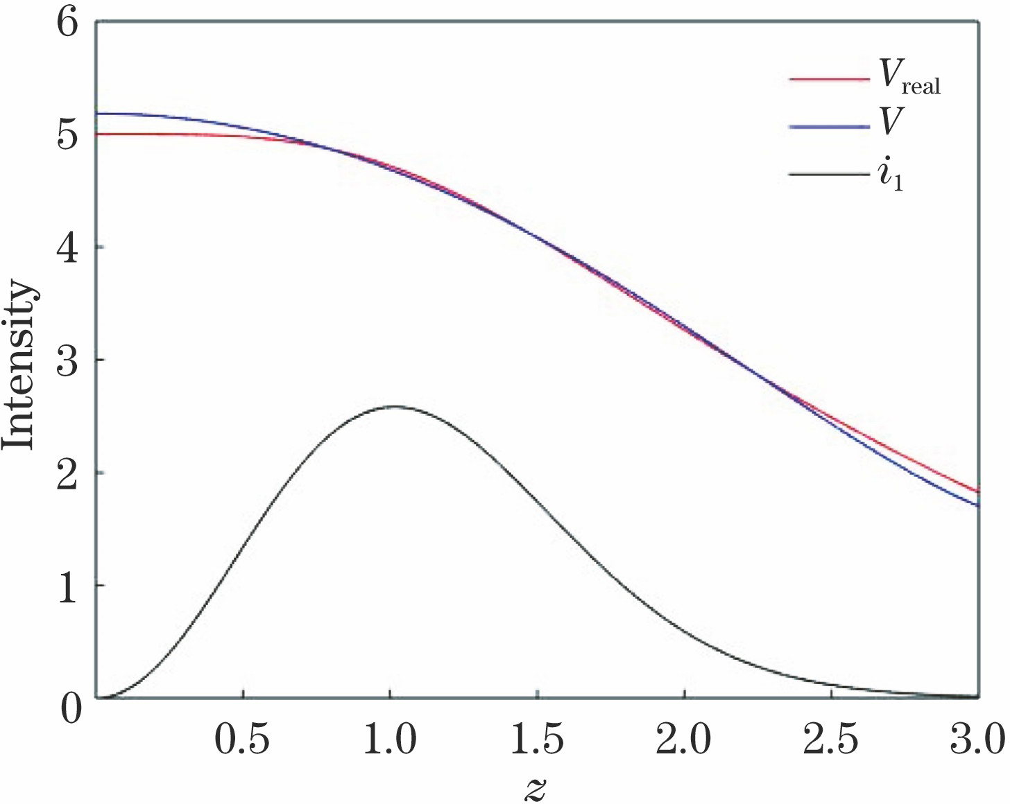
Fig. 1. Fitting diagram of true refractive index and polynomial approximate refractive index in intensity range of vortex soliton solutions with l=1

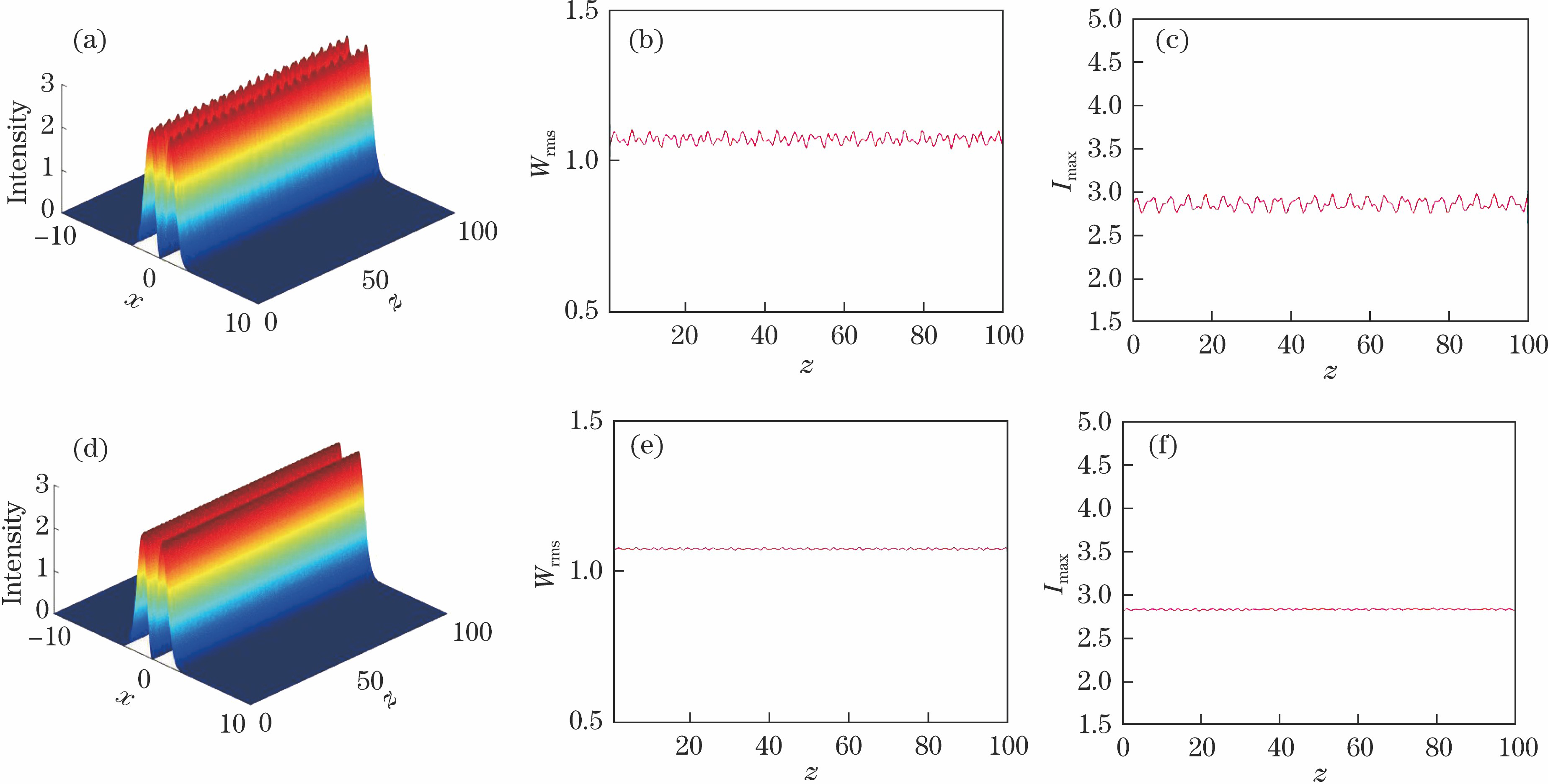
Fig. 2. Comparison of transmission results between ground state solutions and second-order perturbation solutions with l=1. (a) Transmission diagram of ground state solutions; (b) statistical beam width of ground state solutions; (c) maximum intensity diagram of ground state solutions; (d) transmission diagram of second-order perturbation solutions; (e) statistical beam width of second-order perturbation solutions; (f) maximum intensity diagram of second-order perturbation solutions

Fig. 3. Comparison of transmission results between ground state solutions and second-order perturbation solutions with l=2. (a) Transmission diagram of ground state solutions; (b) statistical beam width of ground state solutions; (c) maximum intensity diagram of ground state solutions; (d) transmission diagram of second-order perturbation solutions; (e) statistical beam width of second-order perturbation solutions; (f) maximum intensity diagram of second-order perturbation solutions

Fig. 4. Comparison of transmission results between ground state solutions and second-order perturbation solutions with l=3. (a) Transmission diagram of ground state solutions; (b) statistical beam width of ground state solutions; (c) maximum intensity diagram of ground state solutions; (d) transmission diagram of second-order perturbation solutions; (e) statistical beam width of second-order perturbation solutions; (f) maximum intensity diagram of second-order perturbation solutions

Fig. 5. Comparison of transmission results between ground state solutions and second-order perturbation solutions with l=4. (a) Transmission diagram of ground state solutions; (b) statistical beam width of ground state solutions; (c) maximum intensity diagram of ground state solutions; (d) transmission diagram of second-order perturbation solutions; (e) statistical beam width of second-order perturbation solutions; (f) maximum intensity diagram of second-order perturbation solutions