
Yong Chen, Hongguang Guo, Yapeng Ai. Single Image Dehazing Method Based on Multi-Scale Convolution Neural Network[J]. Acta Optica Sinica, 2019, 39(10): 1010001
- Acta Optica Sinica
- Vol. 39, Issue 10, 1010001 (2019)
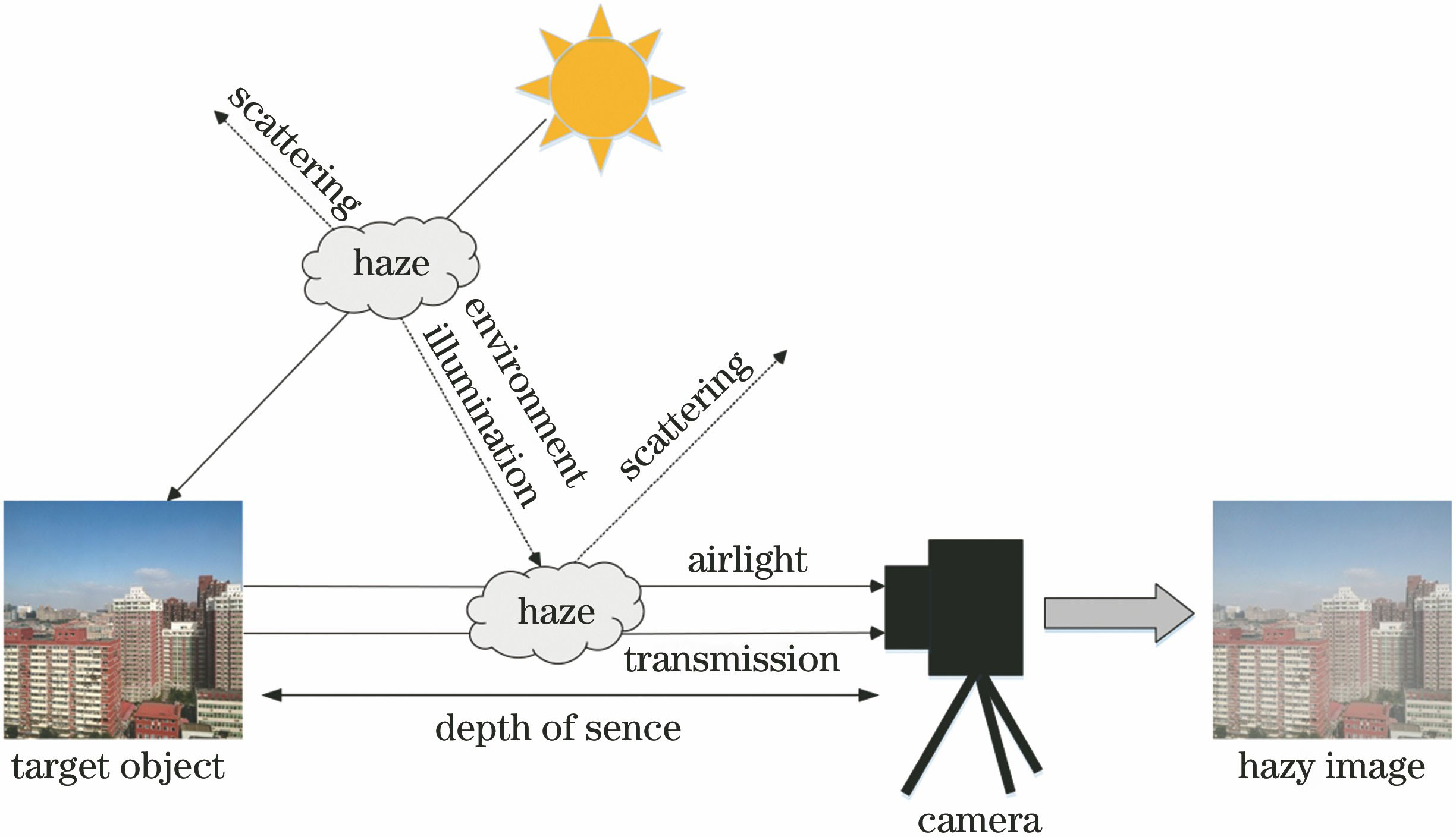
Fig. 1. Physical model of atmospheric scattering
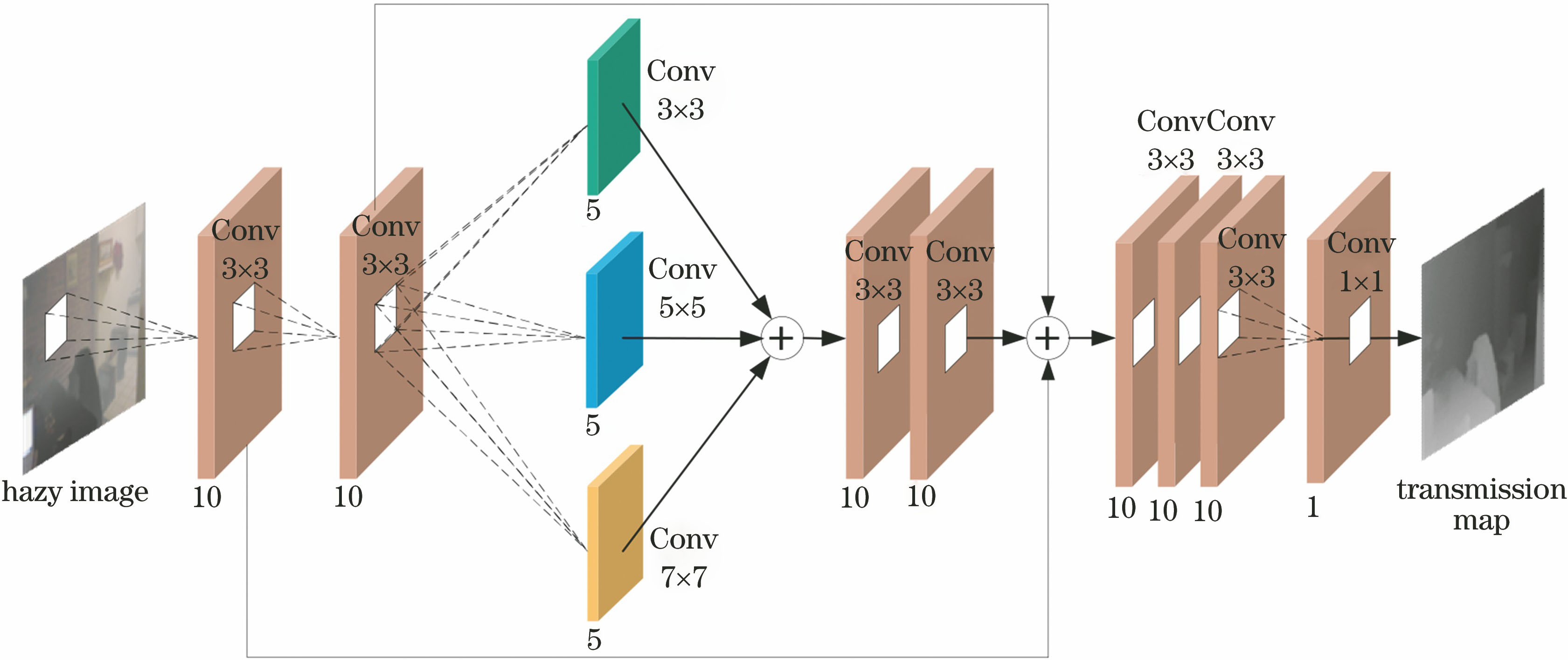
Fig. 2. MSDN model diagram
Fig. 3. Comparison of activation functions. (a) ReLU activation function; (b) PReLU activation function
Fig. 4. Algorithmic steps in this paper
Fig. 5. Training data set. (a) Indoor data set ITS; (b) outdoor data set OTS
Fig. 6. Experimental results of synthesizing hazy images. (a) Hazy image; (b) standard haze-free image; (c) method in Ref. [7]; (d) method in Ref. [11]; (e) method in Ref. [12]; (f) method in Ref. [13]; (g) method in Ref. [14]; (h) proposed method
Fig. 7. Experimental results of real outdoor hazy images. (a) Hazy images; (b) method in Ref.[7]; (c) method in Ref.[11]; (d) method in Ref.[12]; (e) method in Ref.[13]; (f) method in Ref.[14]; (e) proposed method
| ||||||||||||||||||||
Table 1. Parameter table of multi-scale feature extraction kernel
| |||||||||||||||||||||||||||||||||||||||||||||||||||||||||||||||||||||||||||||||||||||||||||||||||||||||||||||||||||||||||||||||||||||||||
Table 2. Analysis of experimental data of synthetic hazy images
| |||||||||||||||||||||||||||||||||||||||||||||||||||||||||||||||||||||||||||||||||||||||||||||||||||||||||||||||||||||||||||||||||||||||||||||||||||||||||||||||||||||||||||||||||||||||||||||||||||||
Table 3. Analysis of experimental data of outdoor hazy images
| |||||||||||||||||||||||
Table 4. Running time of different algorithms for experimental imagess

Set citation alerts for the article
Please enter your email address
© Copyright 2018-2021 | Chinese Laser Press. All Rights Reserved 沪ICP备15018463号-20