Trajectory optimization of hypersonic glide vehicle with minimum total infrared radiation （Invited）

Hui Xu; Guangbin Cai; Chaoxu Mu; Yanhong Zhang; Xin Li

doi:10.3788/IRLA20220194

Journals >Infrared and Laser Engineering >Volume 51 >Issue 4 >Page 20220194 > Article

Infrared and Laser Engineering
Vol. 51, Issue 4, 20220194 (2022)

Trajectory optimization of hypersonic glide vehicle with minimum total infrared radiation （Invited）

Hui Xu¹, Guangbin Cai¹, Chaoxu Mu², Yanhong Zhang³, and Xin Li¹

Author Affiliations

¹College of Missile Engineering, Rocket Force University of Engineering, Xi'an 710025, China

²School of Electrical and Information Engineering, Tianjin University, Tianjin 300072, China

³Beijing Haidian Qinghe Building Ding 7, Beijing 100085, China

show less

DOI: 10.3788/IRLA20220194 Cite this Article

Hui Xu, Guangbin Cai, Chaoxu Mu, Yanhong Zhang, Xin Li. Trajectory optimization of hypersonic glide vehicle with minimum total infrared radiation （Invited）[J]. Infrared and Laser Engineering, 2022, 51(4): 20220194 Copy Citation Text

show less

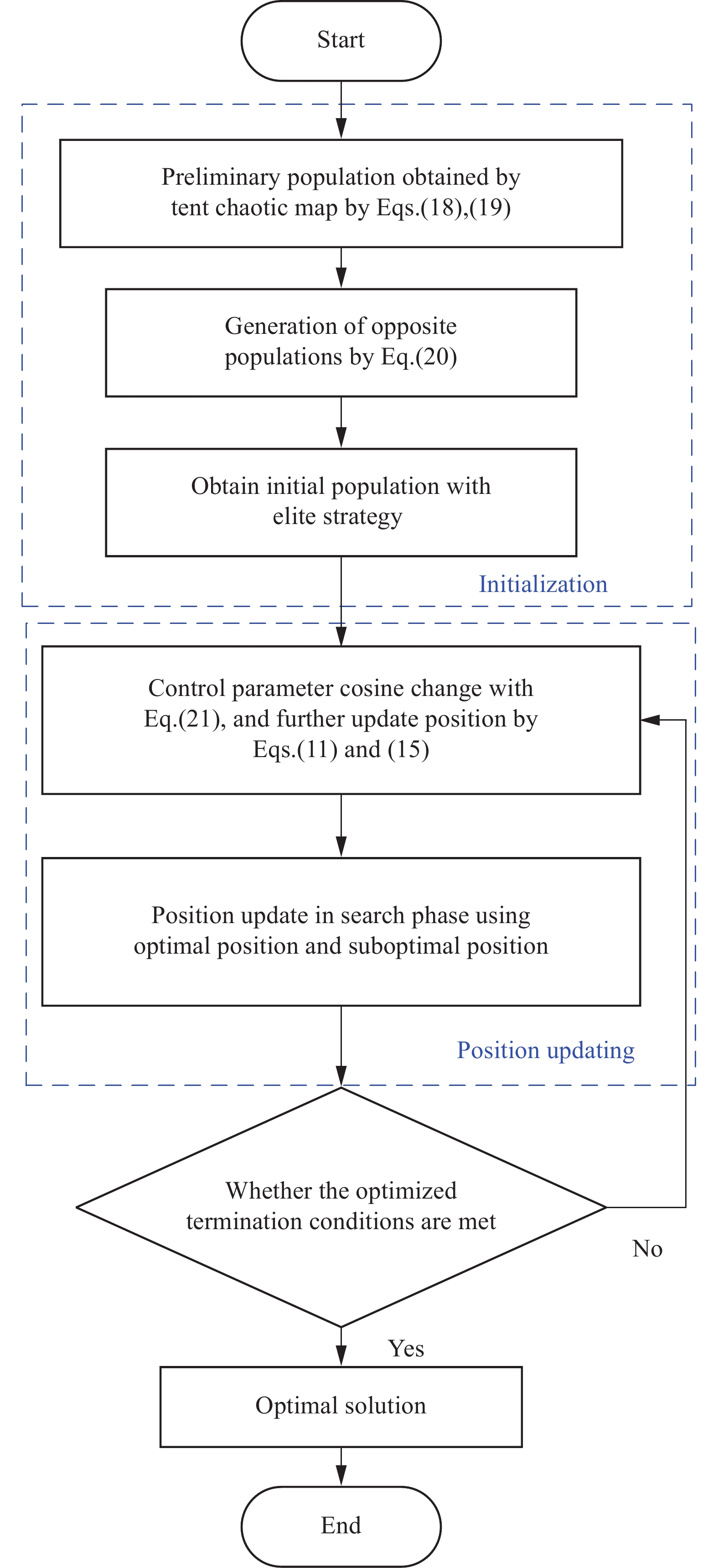
Fig. 1. IWOA flow chart

Download full size | View in the Article

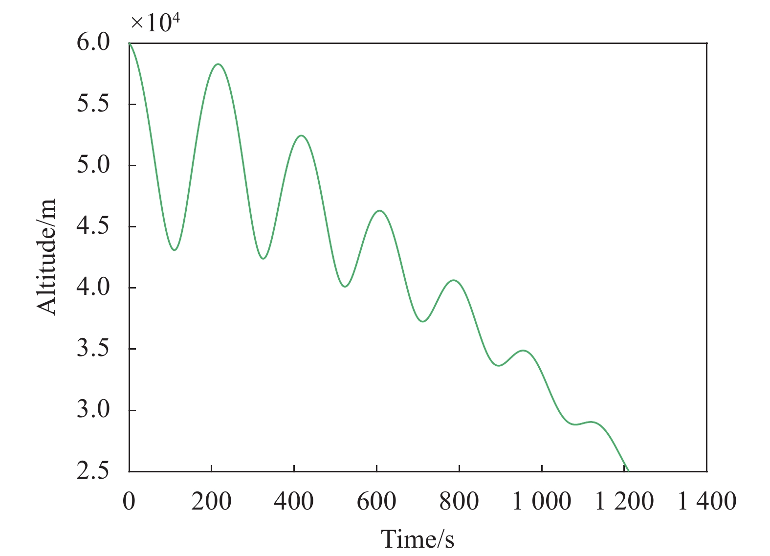
Fig. 2. Time history of the height

Download full size | View in the Article

Fig. 3. Histories of the longitude and latitude

Download full size | View in the Article

Fig. 4. Time history of the velocity

Download full size | View in the Article

Fig. 5. Resistance acceleration reentry corridor

Download full size | View in the Article

Fig. 6. Time histories of the AOA

Download full size | View in the Article

Fig. 7. Time histories of the bank angle

Download full size | View in the Article

Fig. 8. Time histories of temperature on stagnation point

Download full size | View in the Article

Fig. 9. Time histories of the infrared radiation

Download full size | View in the Article

Fig. 10. Time histories of the altitude

Download full size | View in the Article

Fig. 11. Histories of the longitude and latitude

Download full size | View in the Article

Fig. 12. Time histories of the velocity

Download full size | View in the Article

Fig. 13. Resistance acceleration reentry corridor

Download full size | View in the Article

Fig. 14. Velocity histories of the AOA

Download full size | View in the Article

Fig. 15. Velocity histories of the bank angle

Download full size | View in the Article

Fig. 16. Time histories of temperature on stagnation point

Download full size | View in the Article

Fig. 17. Time histories of the infrared radiation intensity

Download full size | View in the Article

Fig. 18. Time histories of the velocity

Download full size | View in the Article

Fig. 19. Time histories of the altitude

Download full size | View in the Article

Fig. 20. Terminal errors of longitude and latitude

Download full size | View in the Article

Fig. 21. Velocity histories of the bank angle

Download full size | View in the Article

Fig. 22. Time histories of temperature on stagnation point

Download full size | View in the Article

Fig. 23. Time histories of the infrared radiation intensity

Download full size | View in the Article

State	Initial condition	Terminal constraint	Other parameters	Value
$ r $/km	60	25	$ {\dot{Q}}_{\text{max}} $/ $ {\text{kW/}}{{\text{m}}^{-{\text{2}}}} $	1200
$ \theta $/(°)	120	160	$ {q}_{\text{max}} $/ ${\text{kPa} }$	400
$ \varphi $/(°)	40	65	$ {n}_{\text{max}} $	6
$ V $/m·s−1	5000	1200	$ {V}_{1} $/m·s−1	$ [4\;000,4\;800] $
$ \gamma $/(°)	−1	-	$ {V}_{2} $/m·s−1	$ [1\;800,4\;000] $
$ \psi $/(°)	40	-	$ \|{\sigma _0}\| $/(°)	$ [0,80] $

Table 1. Simulation scene parameters

View in the Article

Variable	$ {V_1}$/m·s⁻¹	$ {V}_{2} $/m·s⁻¹	$\|{\sigma _0}\|$/(°)	$ J(u)$/kW·sr⁻¹
Value	4000.01	1800.21	41.48	29560.64

Table 2. Optimization results of four algorithms

View in the Article

Algorithms	$ {V_1} $/m·s⁻¹	$ {V_2} $/m·s⁻¹	$\|{\sigma _0}\|$/(°)	$J(u)$/kW·sr⁻¹
IWOA	4000.01	1800.21	41.48	29560.64
WOA	4063.99	1951.63	45.47	34563.88
SSA	4000.52	1800.89	43.54	31268.92
PSO	4135.48	1895.52	47.94	38287.97

Table 3. Simulation results of four algorithms

View in the Article

Terminal errors	IWOA	WOA	SSA	PSO
Altitude/km	0.077	0.84	1.12	0.74
Velocity/m·s−1	0.0086	0.24	97.56	10.50
Longitude/(°)	0.30	0.72	0.86	1.70
Latitude/(°)	0.07	0.19	0.21	0.42
Peak temperature/K	1921.37	2061.98	1977.75	2173.41
Peak radiation/ ${\text{kW} } \cdot {\text{s} }{ {\text{r} }^{ - 1} }$	283.32	368.04	316.12	442.79

Table 4. Comparison of optimization results

View in the Article

Disturbance	$ 3\sigma $values
Altitude/m	200
Longitude/(°)	1
latitude/(°)	1
Velocity/m·s−1	100
Flight path angle/(°)	0.2
Head angle/(°)	0.2

Table 5. Disturbances in the Monte Carlo

View in the Article

Terminal error	Maximum value	Average value	Standard deviation
Altitude/km	0.99	0.71	0.21
Velocity/m·s−1	99.99	94.88	9.68
Longitude/(°)	3.71	1.12	0.42
Latitude/(°)	1.00	0.23	0.20
Peak temerature/K	2213.60	1962.54	178.02
Peak radiation/ ${\text{kW} } \cdot {\text{s} }{ {\text{r} }^{ - 1} }$	471.73	314.34	52.20
Total radiation/ ${\text{kW} } \cdot {\text{s} }{ {\text{r} }^{ - 1} }$	40278.91	31592.07	3516.83

Table 6. Simulation results of the Monte Carlo

Download Citation

Save the article for my favorites

Paper Information