Fig. 1. CPC longitudinal cross section^[12]

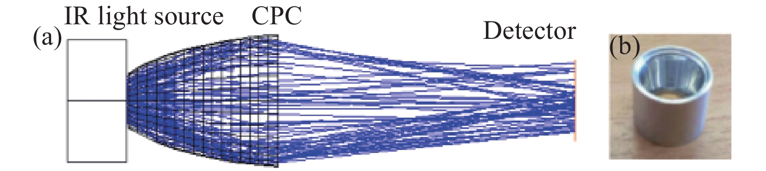
Fig. 2. (a) Optimization results of the CPC focusing system; (b) Aluminum CPC

Fig. 3. (a) Signal acquisition system (gas chamber) with CPC; (b) Respiratory CO₂ monitoring system; (c) Schematic diagram of the main parts of the monitoring system

Fig. 4. (a) Straight cylinder concentrator; (b) Cone concentrator; (c) compound parabolic concentrator ray trace using ZEMAX, and samples of them; (d) Photoconductive infrared detector of the chamber

Fig. 5. (a) CMOS detector(Point Grey Research, Inc) (left) and IR source EMIRS200（Axetris）(right); (b) Environment of CPC verification experiment

Fig. 6. Calibration experiment environment diagram

Fig. 7. When the CPC and the detector are at different distances, (a) Spot pattern on the detector obtained by ZEMAX simulation; (b)Spot pattern captured by the CMOS detector in the verification experiment；(c) Comparison of the normalized light spot cross-section brightness distribution between the simulation results (silver) and experimental results (orange) at different distances between the CPC and the detector

Fig. 8. (a)Straight cylinder concentrator, (b)cone concentrator , (c)light distribution of compound parabolic concentrator on the signal channel detector

Fig. 9. Relationship between the output signals of three systems corresponding to the CO₂ concentration in the range of 10 000 ppm to 73 000 ppm CO₂ concentration

Fig. 10. CO₂ waveform

Table 1. Input parameters in ZEMAX

Table 2. Optimized parameters of CPC

Table 3. Optical efficiency simulation results of three structures

Table 4. Third-order polynomial fitting coefficient and calibration coefficient of system output and CO₂ concentration

Table 5. Signal-to-noise ratio of the monitoring system after installing three structures