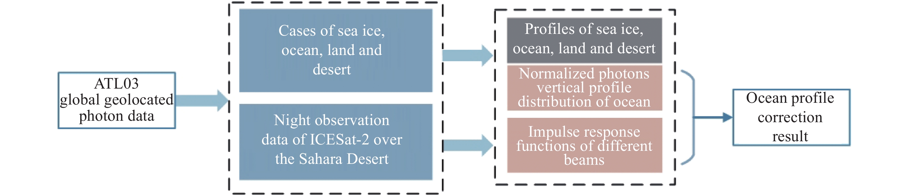
Fig. 1. Flow chart of ATLAS/ICESAT-2 data preprocessing and calibration

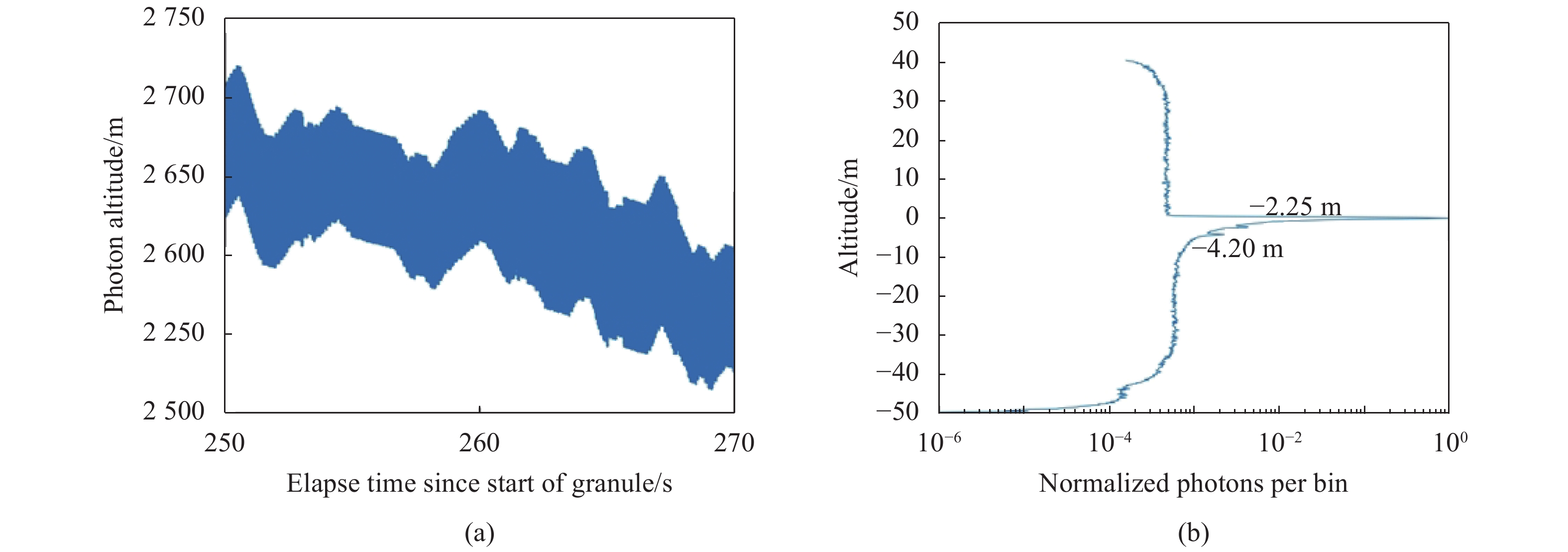
Fig. 2. (a) Photon distribution from sea ice surface (Height of each received photon, relative to the WGS-84 ellipsoid); (b) The photons vertical profile distribution, x-axis is normalized photon counts per bin and y-axis is altitude in meter. The altitude of peak surface return is set to 0 meter in (b)

Fig. 3. (a) Photon distribution from ocean surface (Height of each received photon, relative to the WGS-84 ellipsoid); (b) The photons vertical profile distribution, x-axis is normalized photon counts per bin and y-axis is altitude in meter. The altitude of peak surface return is set to 0 meter in (b)

Fig. 4. (a) Photon distribution from land surface (Height of each received photon, relative to the WGS-84 ellipsoid); (b) The photons vertical profile distribution, x-axis is normalized photon counts per bin and y-axis is altitude in meter. The altitude of peak surface return is set to 0 meter in (b)

Fig. 5. (a) Photon distribution from desert surface (Height of each received photon, relative to the WGS-84 ellipsoid); (b) The photons vertical profile distribution, x-axis is normalized photon counts per bin and y-axis is altitude in meter. The altitude of peak surface return is set to 0 meter in (b)

Fig. 6. Impulse response curves of six beams, in which the green curve is the impulse response function under the beam

Fig. 7. Impulse response of six beams

Fig. 8. Location of marine data used in this paper

Fig. 9. (a) Photon distribution from ocean surface (Height of each received photon, relative to the WGS-84 ellipsoid); (b) The photons vertical profile distribution, x-axis is normalized photon counts per bin and y-axis is altitude in meter. The altitude of peak surface return is set to 0 meter in (b)

Fig. 10. (a)-(f)：Calibration results were obtained by using impulse response models under six beams, where the black curve represents the observed ocean profile, the blue curve represents the impulse response model, and the red curve represents the correction results

Fig. 11. The correction results of the observed ocean profile, where the black curve represents the observed ocean profile and the other color curve represents the deconvolution results of different beams

Table 1. Configuration parameters of ATLAS/ICESat-2^[2]